Honeywell Home resideo EW500 Series Manual

EW500 Series
Installation and Setup Instructions Instrucciones de instalación y configuración Instrukcja instalacji i obsługi
Keep instructions for later use! Heat Metering
¡Guarde las instrucciones para un posterior uso! Medición de calor
Instrukcjê nale¿y zachowaæ na potrzeby póŸniejszego u¿ycia! Pomiar ciep³a
EW5001CD0100
Flow sensor
on supply pipe
Pt500 (EN 60751)
1...180° C
3...170° C
1 dm
3
/imp
IP54, E1, M1
Class C (
EN 1434 )
M14
SK 14-029 MI-004
FAUN D2040MB
Manufactured by Apator
00060514
1446
32301258-001A

2 MU1H-0511GE23 R0720
GB
1 Installation of the calculator . . . . . 3
2 LCD screen . . . . . . . . . . . . . . . . . 4
3 Configuration of the calculator from
the menue . . . . . . . . . . . . . . . . . . 4
4 Electrical connections . . . . . . . . . 5
5 Dimensions . . . . . . . . . . . . . . . . . 9
6 Error code description . . . . . . . . . 9
7 Display sequence. . . . . . . . . . . . 10
E
1 Instalación de el calculador . . . . 21
2 Pantalla LCD . . . . . . . . . . . . . . . 21
3 Configuración de el calculador
desde el menú . . . . . . . . . . . . . . 22
4 Conexión eléctrica . . . . . . . . . . . 23
5 Dimensiones . . . . . . . . . . . . . . . 27
6 Descripción del código de error . 27
7 Secuencia del display . . . . . . . . 27
PL
1 Montażprzelicznika . . . . . . . . . . 28
2Wyświetlacz LCD . . . . . . . . . . . . 28
3 Konfiguracja przelicznika z poziomu
menu . . . . . . . . . . . . . . . . . . . . . 29
4 Podłączenia elektryczne . . . . . . 30
5 Wymiary . . . . . . . . . . . . . . . . . . . 34
6 Opis kodów błędów . . . . . . . . . . 34
7Wyświetl sekwencję. . . . . . . . . . 34

GB
MU1H-0511GE23 R0720 3
1 INSTALLATION OF THE CALCULATOR
1.1 Installation of the calculator on the wall
1. Remove the A mounting base (Fig. 1) from the calculator by moving it
in the direction opposite than indicated by the arrows on it
2. Mark the holes for mounting studs on the wall according to the
dimensions shown in Fig. 2 or by holding the mounting base to the wall
3. Drill the holes for the mounting studs using ø6 drill applicable to the wall
material
4. Place the mounting studs included in the set in the drilled holes
5. Hold the A mounting base to the wall in such a way that the holes in the
base match the mounting studs in the holes
6. Attach the base to the wall using the screws included in the set
7. Slide the calculator onto the installed mounting base as shown in Fig. 3
8. Unscrew the B screws holding the calculator cover (Fig. 4)
9. Remove the C cover of the calculator (Fig. 5)
10. Connect electrical wires as described in the section "Electrical
connections"
11. Place the C cover back on the mounting base of the calculator
12. Screw the C cover to the mounting base using B screws
13. Place the seals (Fig. 6 – wire, Fig. 7 – sticker)
1.2 Installation of the calculator on the ultrasonic
transducer
1.2.1EW400 Ultrasonic Flow Meter
1. Remove the A mounting base (Fig. 1) from the calculator by moving it
in the direction opposite than indicated by the arrows on it
2. Place the calculator on the mounting slot of ultrasonic transducer (Fig.
8)
3. Move the calculator in the direction of cable holes until it clicks on the
transducer
4. Follow the instructions in points 8-13 in case of mounting the calculator
on the wall
1.2.2Ultraflow transducers
1. Remove the A mounting base (Fig. 1) from the calculator by moving it
in the direction opposite than indicated by the arrows on it
2. Place the mounting base on the mounting slot of ultrasonic transducer
3. Move the mounting base bracket in the direction opposite than
indicated by the arrows on it until it clicks on the transducer
4. Follow the instructions in points 7-13 in case of mounting the calculator
on the wall
Fig. 1
Fig. 2 Fig. 3
Fig. 4
Fig. 5 Fig. 6
Fig. 7 Fig. 8 Ultrasonic transducer
51-931090-001
TOP
70,5 mm
73,5 mm
4 x 4,5 mm
36,5 mm
39,5 mm
53,5 mm
B
B
B
only IP68
B
only IP68
C
A
B
CD
przetwornik
ultradźwiękowy

GB
4 MU1H-0511GE23 R0720
2 LCD SCREEN
Description of the symbols displayed on the calculator screen (Fig.9) is
presented below.
1. Symbol indicating the display of volume or flow value, as well as
additional input values when displayed along with the symbol in the field
no. 2
2. Symbol of additional input or tariff, indicating the display of data
(register or configuration value) for additional input, symbols:
or the values associated with tariffs, symbols: 1, 2.
3. Symbol of instantaneous/minimum/maximum/average or tariff value,
indicating the display of one of the following values:
– instantaneous value: for the flow and power,
– minimum value:
– maximum value:
– average value:
– tariff value : displayed together with the symbol in the field no.
2, indicating the tariff number.
4. Symbol of power supply temperature, displayed for the instantaneous,
average or peak value, as well as archived power supply temperature
5. Symbol of temperature difference, indicating together with symbols 4
and 6 the display of temperature difference
6. Symbol of return temperature
7. Symbol of cold, displayed for the values of cold registers: energy and
volume, as well as on the screen of temperature difference measured
in time, when the conditions of cold measurement are met
8. Symbol of failure, indicating the occurrence of failure. The symbol is
displayed on the main screen and on the screens associated with that
failure, where in the field no. 18 a message on error type is additionally
displayed
9. Symbol of time, displayed on date and current time screens for the date
and time values associated with archived data and working time
10. Symbol indicating the access level to the configuration of calculator
(displayed on all screens during access unlocking). The blinking symbol
indicates the access to metrological settings, whereas steady light
symbol – access to user settings
11. Symbol of return flow, indicating the flow at variance with the proper
direction. Available only for flow transducers with digital communication
12. Symbol of flow, indicating flow in the proper direction
13. Symbol of low battery, displayed along with the symbols 14 and 15,
indicates the type of low battery (displayed on all screens during the
occurrence of failure) or the type of battery, for which the voltage is
displayed in the service menu
14. Symbol of main battery, displayed along with the symbol 13, indicates
the values or signals the failure of the main battery
15. Symbol of backup battery, displayed along with the symbol 13, indicates
the values or signals the failure of the backup battery
16. The main display field, 8-digit field for displaying values and
configuration data of the calculator
Fig. 9
17. Symbol of the archive, displayed with the symbol 19, 21, 22, 23, 24 or
25, indicates the type of archived data displayed
18. Additional display field, 4-digit field for displaying additional descriptions
of the values displayed in the main field, the error type and the current
or archived time on selected screens
19. Symbol of daily data, indicating the display of archived data from the
daily archive
20. Symbol of optical port activity, appears when the optical port is active
and communication is possible
21. Symbol of monthly data, indicating the display of data from the monthly
archive
22. Symbol of annual data, indicating the display of data from the annual
archive
23. Symbol of hourly data, indicating the display of archived data from the
hourly archive
24. Symbol of minute-based data, indicating the display of data from the
minute-based/configurable archive
25. Symbol of tariff data, indicating the display of data from the tariff archive
26. Decimal symbol, indicating the decimal part of a value or separating
rating different values
27. Decimal separator symbol, highlighting the decimal part of a value
28. Symbol of impulse frequency, indicating the impulse frequency unit
29. Unit field, indicating the unit of value displayed in the main field,
available units of energy, volume, flow, power and time
3 CONFIGURATION OF THE
CALCULATOR FROM THE MENUE
The calculator allows for a manual configuration of selected parameters from
the menu.
You can set parameters such as date, time, network settings and additional
input settings.
Configuration possibility is secured by a configuration jumper available after
opening the casing (Fig. 10).
Fig. 10
Upon pressing and holding the jumper for 1 second, the configuration group
selection screen is automatically displayed (06).
Configuration group is available for 5 minutes after using the jumper or after
recent activity in this group.
After this time, the display automatically returns from the configuration group
to the main energy; to enable configuration group, use the jumper again.
When the possibility of configuration is active, at any time it is possible to exit
and re-enter the group in a standard way.
Upon moving to the configuration menu the current calculator configuration
is read and then displayed during editing.
Navigating between screens of the configuration group takes place in a
standard way.
Fig. 11
,
,
,
,
,
1 2 3 4 5 6 7 8 9 10 11 12 13 14 15
16 17 18 19 20 21 22 23 24 25 26 27 28 29
Configuration jumper
P1 P2

GB
MU1H-0511GE23 R0720 5
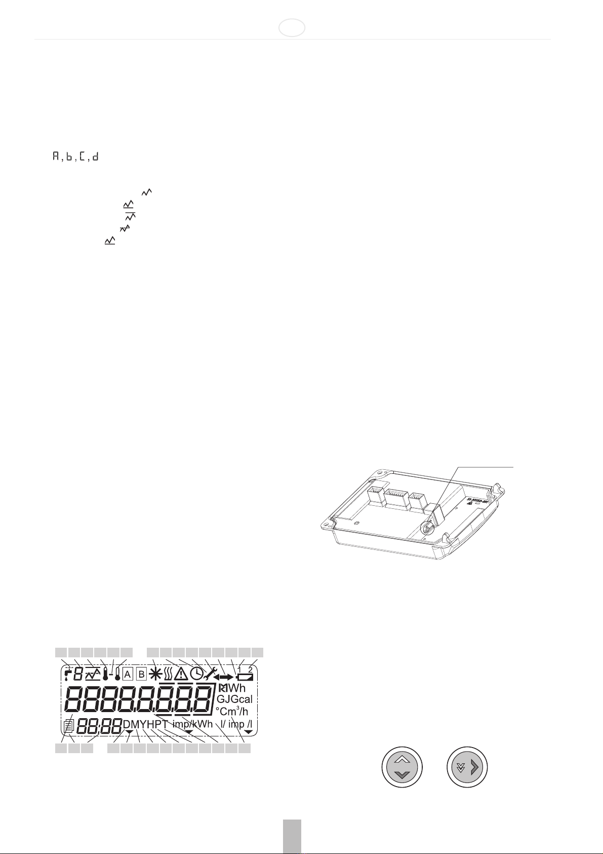
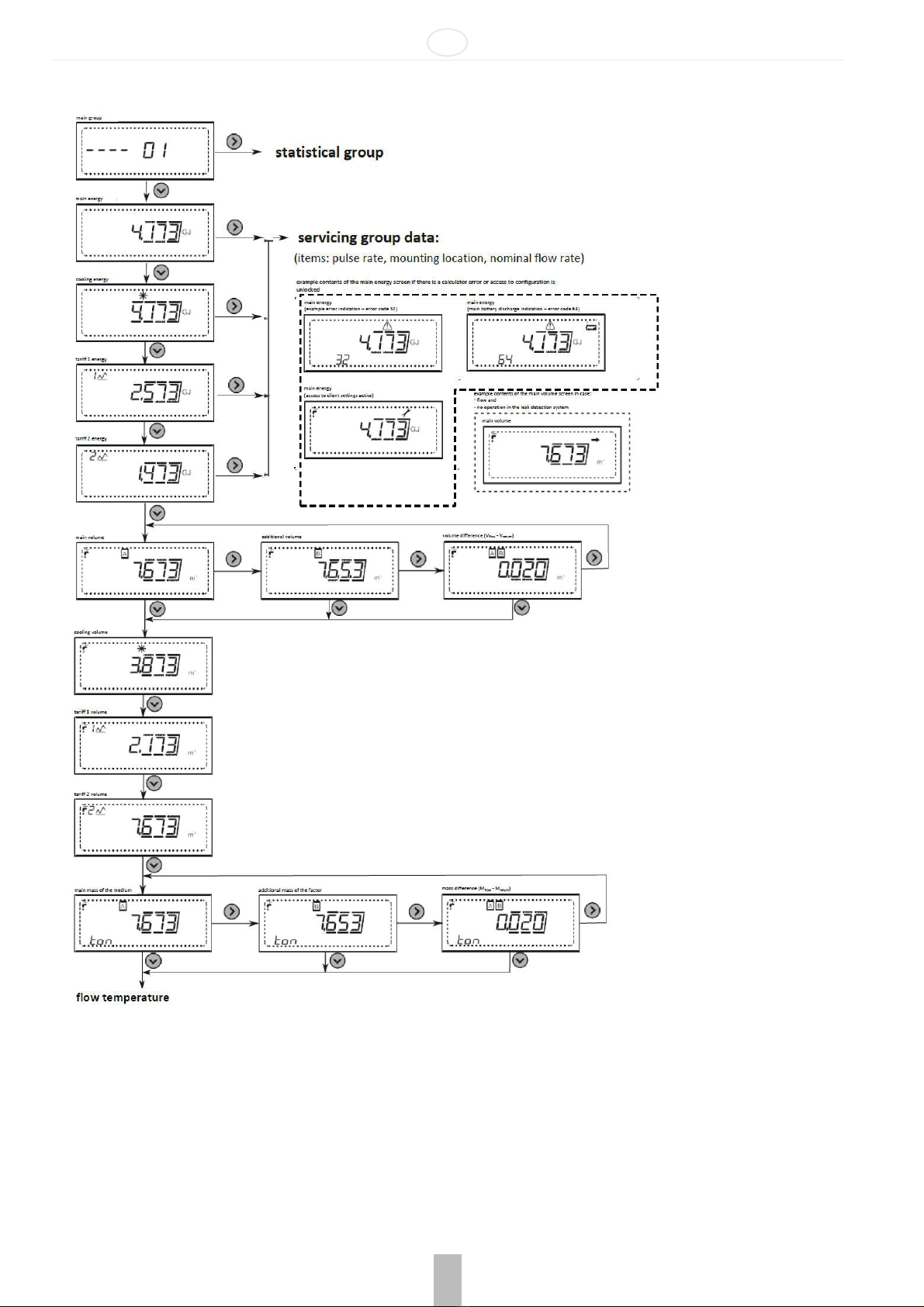
3.1 Numeric value editing
To start editing a numeric value, briefly push the P2 button at the time of its
display (Fig. 11).
The first digit of the edited value will start flashing.
By briefly pushing the P2 button, set the appropriate value; to move to the
next digit editing, briefly push the P1 button (Fig. 11).
To exit the editing mode of a given value, go to the last editable digit and
briefly push the P1 button once more.
As a result, the last digit will stop flashing and the screen will return to the
value display mode, after which it will be possible to select the next value to
edit.
In this way it is possible to configure the following parameters in the
calculator:
• date and time,
• network address and customer ID,
• impulse frequency and serial number for additional inputs,
• initial value of the meter for additional inputs.
3.2 Date and time editing
Configuration of date and time takes place on the same menu screen.
To edit the date, briefly push the P2 button when in the settings menu.
Editing begins with the year, each next push of the P1 button enables the
editing of the month, day, hour and minutes.
Set date and time are saved in the calculator upon finishing the editing of the
last digit (tens of minutes).
3.3 Additional input type editing
To change the type of the additional input, briefly push the P2 button when
displaying the impulse input type screen.
As a result, the input type will be changed to another type available.
Depending on the input number, it is possible to set the following types of
inputs:
• inactive input,
• impulse input with impulse frequency: dm3/imp, imp/dm3, imp/kWh,
• alarm input,
• input for digital communication with transducer.
Note: In case of setting the output type other than an impulse one in the menu, the impulse
frequency and serial number settings for the given input are not displayed.
3.4 Confirmation of the edited parameters
When setting date and time, the parameters in the calculator are updated
immediately after the end of editing.
In order to confirm the remaining values, go to the last screen – confirmation
of configuration group changes.
If there have been changes made to the current configuration, the APPLY
option will appear on the screen.
To save the changed configuration, push and hold the P2 button until the
screen displays "No rConF".
This means that the calculator is already configured in accordance with the
data entered in the configuration menu.
Note: If the configuration group is abandoned without the implementation of the operation
described above, introduced settings will not be saved in the calculator.
4 ELECTRICAL CONNECTIONS
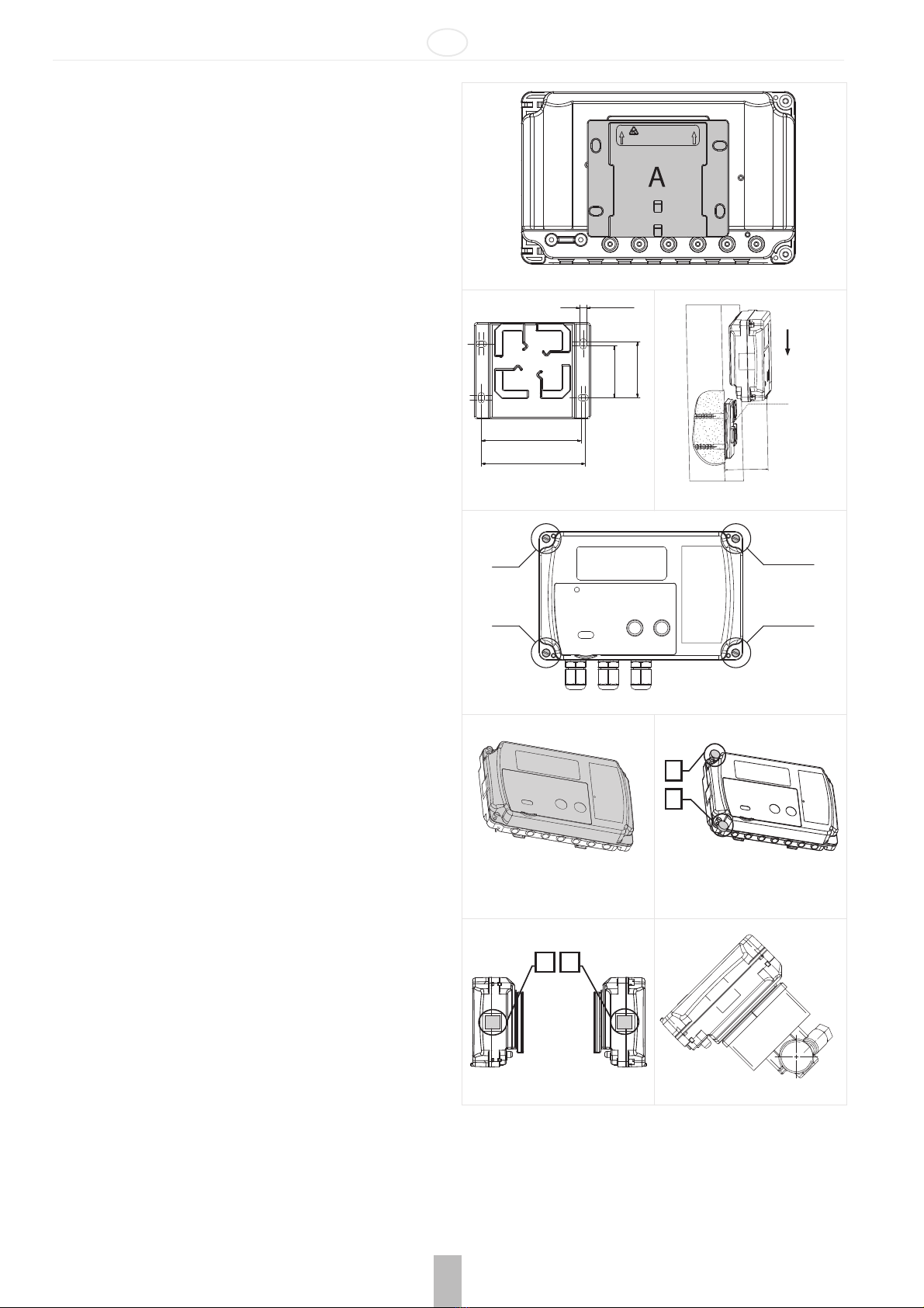
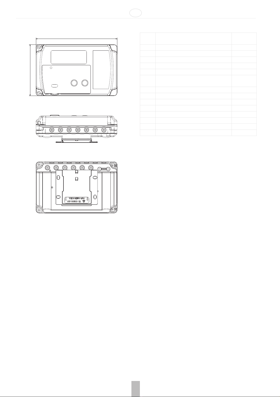
To make electrical connections, remove the C cover of the calculator (Fig. 5).
The removal method is described in the section "Installation of the
calculator".
4.1 Connecting the temperature sensors
The calculator can work with two types of temperature sensors (Pt500 and
Pt1000), but for each of them there is a separate design of the main plate of
the calculator.
Temperature measurement can be performed using the Pt500 or Pt1000
sensors, both 2- and 4-wire.
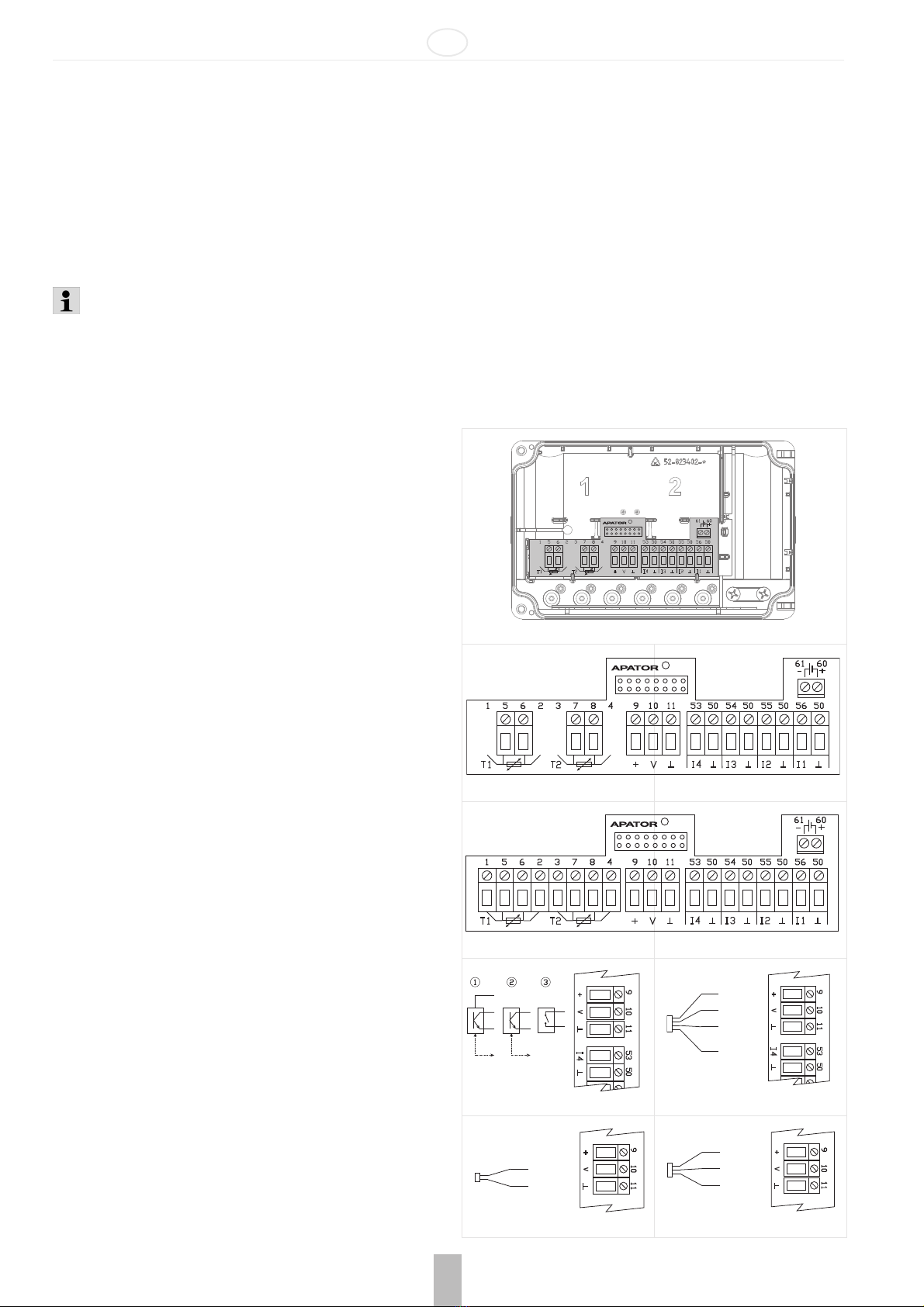
Depending on the number of temperature sensor connection wires, the
calculator connection strips are available in two versions (Fig. 12):
• calculator with a strip for 2-wire temperature sensor, a strip for the
connection of the main flow transducer and a strip for the connection of
4 additional devices (Fig. 13),
• calculator with a strip for 4-wire temperature sensor, a strip for the
connection of the main flow transducer and a strip for the connection of
4 additional devices (Fig. 14).
When measuring with 2-wire sensors (Fig. 13), the T1 sensor (power supply
temperature) must be connected to the connector marked with numbers 5, 6,
whereas the T2 sensor (return temperature) – to connector no. 7, 8.
When measuring with 4-wire sensors (Fig. 14), the T1 sensor must be
connected to the connector marked with numbers 5, 6 and 1, 2, whereas the
T2 sensor – to connector no. 7, 8 and 3, 4.
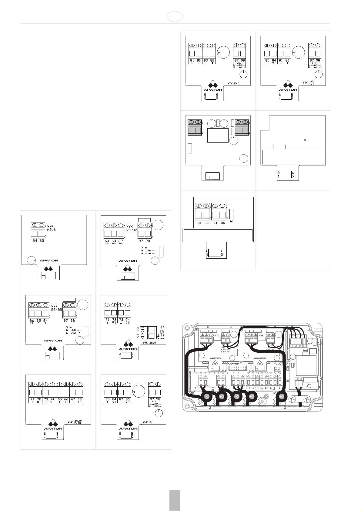
4.2 Connecting the flow transducer
The connection of the main flow transducer is made through a 3-terminal
connector, marked with numbers:
30. power supply output for flow transducer (from the main power source)
31. signal input for the flow transducer
32. signal reference input for the flow transducer
What is more, there is a possibility of connecting the flow transducer
communication cable to the signal input – the fourth additional input (only if
it is configured as a input of digital communication with the transducer).
Fig. 15 shows the method of connecting flow transducers with open collector
output for the transducer requiring power supply from the calculator (1), open
collector output (2) and normally open contact output (3).
In the case of ultrasonic transducers with a 4-wire connection (e.g.
Sharky 473) the fourth wire (yellow) can be connected only if input I4
is configured as a digital communication with the transducer.
Otherwise, do not connect this cable. Incorrect connection may result
in premature battery wear.
Connecting the flow transducer to the NC transmitter
•connection polarity arbitrary (Fig. 16)
Connecting Sharky 473 ultrasonic transducer (Fig. 17)
Connecting Ultraflow ultrasonic transducer (Fig. 18)
4.3 Connecting the additional flow sensor
The additional flow sensor may be used to detect leaks of the systems
operating in the closed system. It should be connected to the additional input
3. The sensor should be connected with the 2 terminal connector marked
with the following numbers:
54 - signal input for the additional flow sensor,
50 - additional flow sensor signal reference output.

GB
6 MU1H-0511GE23 R0720
Moreover, you can also connect the sensor communications and power
supply input:
9 - power supply output for the flow sensor (from the main power supply
source),
55 - signal input (only if it is configured as a input of digital communication
with the transducer) to communicate with the additional flow sensor
(additional input 2).
Please refer to the diagram below to connect the additional flow sensor with
the open collector output for the sensor with the required power supplied
from the calculator (1), open collector output (2) and the normally closed
contact output (3).
In the case of ultrasonic transducers with a 4-wire connection (e.g.
Sharky 473) the fourth wire (yellow) can be connected only if input I2
is configured as a digital communication with the transducer.
Otherwise, do not connect this cable. Incorrect connection may result
in premature battery wear.
4.4 Connecting external power supply
The calculator can be powered from 230VAC or 24VAC power adapter, as
well as using AA batteries, two AA or C batteries mounted on a separate
plate or D battery mounted directly in the base.
Opening the cover provides direct access to the main battery or power
adapter (Fig. 19).
If you are replacing the D battery on your own, pay attention to how it is
mounted in the casing, the positive pole should be facing the upper edge of
the casing.
Each battery or power adapter has cables to be connected to the calculator.
Main power supply must be connected on the terminal block (Fig. 12) to the
connector marked with numbers: 60 – positive pole, 61 – negative pole.
In case of calculator equipped with power supply: the power adapter should
be connected to the ~230 V power supply and to the terminals marked with
numbers 27 and 28 (Fig. 20); for the 24 V power adapter the ~24 V power
should be supplied to terminals marked with numbers 97, 98 (Fig. 21).
The power adapter has two sets of terminals marked with numbers 95 and
96, allowing for the supply of power to interchangeable communication
modules (terminals on modules marked with numbers 97 and 98).
The electrical connection of power adapter should be performed by a
properly licensed person.
4.5 Connecting additional input signals
Each version of the terminal block has 4 additional inputs.
Each of the inputs marked I1 (terminal no. 56 and 50), I2 (terminal no. 55 and
50), I3 (terminal no. 54 and 50), I4 (terminal no. 53 and 50) can operate as
an impulse input, the I3 input can additionally serve as an alarm input, and
the I4 input can be used for digital communication with the flow transducer.
Each input has two terminals, marked as follows:
• signal input (terminal no. 56, 55, 54, 53)
• reference input for additional input, each input has a separate terminal
for reference signal connection (terminal no. 50)
Fig. 22 shows the signal connection method for a sample additional input, for
a device with output type: open collector (1), normally open contact (2).
4.6 Installation of additional modules
The calculator allows you to install up to two independent additional modules:
• M-Bus
• RS232
• RS485
• impulse outputs (2x OB, OC or OD class output)
• impulse inputs and outputs (2x OB, OC or OD class output and 2x IB or
IC class input)
• analogue outputs (2x 4-20 mA or 0-10 V output)
• LonWorks
• RF module for IMR telemetry systems (AIUT)
• Wireless M-Bus RF module
Fig. 23 shows the place and method of additional module installation.
Modules can be installed in any connector except for RF modules, which can
only be fitted in the connector marked with number 1 (Fig. 12).
4.7 Installation of the M-Bus module (module code: 001)
M-Bus module is powered from the M-Bus network and galvanically isolated
from the calculator using optical isolation. The module supports primary,
secondary and extended secondary addressing. The M-Bus signals are
connected through the inputs marked with numbers 24,25 (Fig. 24).
Fig. 12
Fig. 13
Fig. 14
Fig. 15 Fig. 16
Fig. 17 Fig. 18
BROWN
WHITE
BLUE
YELLOW
BROWN
WHITE
RED
YELLOW
BLUE

GB
MU1H-0511GE23 R0720 7
4.8 Installation of the RS 232 module (module code: 003)
The RS 232 module requires an external power source.
It is galvanically isolated from the calculator using optical isolation.
The module can be powered by AC or DC voltage.
The power source is connected through terminals no. 97, 98, the polarity of
the connected power supply is arbitrary.
The communication cables are connected through the following terminals: 64
– signal ground, 63 – TxD module output, 64 – RxD module input (Fig. 25).
4.9 Installation of the RS 485 module (module code 003)
The RS 485 module requires an external power source.
It is galvanically isolated from the calculator using optical isolation.
The module can be powered by AC or DC voltage.
The power source is connected through terminals no. 97, 98, the polarity of
the connected power supply is arbitrary.
The communication cables are connected through the following terminals: 86
– signal ground, 84 – A input/output (inverting), 85 – B input/output (non-
inverting) (Fig. 26).
4.10Installation of the impulse input/output module
There are two types of impulse I/O modules.
Modules can be powered, depending on the version, from the calculator or
external power source.
1. module with 2 impulse outputs (Fig. 27, module code: 016): impulse
outputs can operate in different classes: OB, OC and OD (according to
PN-EN 1434-2). Due to the high average power consumption is
recommended to use the module versions with external power supply.
In each case, the outputs are galvanically isolated from the calculator
2. module with 2 outputs + 2 impulse inputs (Fig. 28, module code: 080):
outputs for the I/O module are the same as for the 016 module. Inputs
can operate in IB or IC class (according to PN-EN 1434-2). In each
case, the inputs and outputs are galvanically isolated from the
calculator
The type and resolution of each impulse output can be freely configured. The
output generates impulses whose number is proportional to the increase in
energy or volume (main, additional or tariff), with one of three resolutions:
0.1, 1, 10.
The external power source is connected through terminals no. 97, 98, the
polarity of the connected power supply is arbitrary.
The impulse inputs are connected through terminals no. 65, 66 and 67, 68,
whereas the signal from the impulse outputs – through terminals no. 71, 72
and 73, 74.
4.11Installation of the 2 analogue output module (module
code: 256)
Analogue output module requires an external power supply and has a
galvanic isolation between the calculator and the module.
The module is available in three versions with two current outputs 0/4 ... 20
mA, two voltage outputs 1 ... 10 V or one current and one voltage output.
The analogue outputs can be freely configured to expose a condition
proportional to the instantaneous value of: the flow, power, power supply
temperature, return or temperature difference.
Analogue output status is updated at every determination of instantaneous
values, i.e. every 10 seconds for normal operation with non-zero flow.
Power is supplied to the module through terminals no. 97 and 98. Analogue
output terminals, depending on the version, are described as follows for a
specific version:
1. 2x voltage output (Fig. 29):
– output 1 – terminal 87, reference for output 1 – terminal 88,
– output 2 – terminal 89, reference for output 2 – terminal 90,
2. 2x current output (Fig. 30):
– output 1 positive terminal – 80, negative terminal – 81,
– output 2 positive terminal – 82, negative terminal – 83,
3. 1x current output + 1x voltage output (Fig. 31):
– output 1 (voltage output) – terminal 87, reference for output 1 –
terminal88,
– output 2 (current output) positive terminal – 82, negative terminal
– 83.
Note: If the module is powered from the calculator's power adapter, due to the maximum
load pf power adapter it is possible to install up to one analogue module.
4.12Installation of the LonWorks module
The LonWorks module (Fig. 32) requires an external power source. The
module can be supplied with direct current at a voltage range of 9-24 V.
Power source is connected by means of a pair of terminals located in the
upper right part of the module designated as B.
The positive terminal is marked as Vcc, whereas the negative pole – as GDN.
Communication cables are connected by means of a pair of terminals located
in the upper left part of the module designated as A – the polarity is arbitrary.
Fig. 19
Fig. 20 Fig. 21
Fig. 22
Fig. 23

GB
8 MU1H-0511GE23 R0720
4.13Installation of the Wireless M-Bus module
The Wireless M-Bus module (Fig. 33) is battery-powered and has its own
antenna, so for the purpose of proper operation of the module, just put it in
the appropriate connector.
Note: Wireless M-Bus modules can be mounted only in the connector marked with number
1 (Fig. 12).
4.14Installation of IMR module (APAT 13x2)
There are three types of IMR modules (Fig. 34): with radio interface (APAT
1312), with radio and cable interface (APAT 1322), with cable interface (APAT
1332).
Modules can be powered, depending on the version, from the calculator or
external power source.
Cable interface (terminal no. 34 and 35) can be used to connect an active
AMPLI antenna – cable order does not matter. For the connection of external
power source (in the range of 4-16 V or stabilised 3.6 VDC) the following
terminals are used: 31 – positive pole, 32 – negative pole.
The module supplied by the manufacturer with its own power supply is in the
sleep mode.
The APAT 13x2 module can be activated using the SW1 diagnostic button
(push and hold the button for 5 to 7 seconds, then let go). If APAT 13x2 is a
version without its own power supply or if the system is awake, push and hold
the diagnostic button for 5 seconds to check the operating mode. Correct
operation is signalled with 4x flash of the LED.
Note: IMR modules can be mounted only in the connector marked with number 1 (Fig. 12).
4.15Cable lining inside the calculator
The calculator has been designed to assist you in the installation process as
much as possible. In the base of the device there are special "tunnels" that
help in connection cable lining. The IP54 version of the calculator also
features special pins preventing the cable from being ripped out. In IP65 and
IP68 models this task is performed by cable grommets.
Fig. 35 shows how cable is to be lined inside the device
Fig. 24 Fig. 25
Fig. 26 Fig. 27
Fig. 28 Fig. 29
Fig. 30 Fig. 31
Fig. 32 Fig. 33
Fig. 34
AB
GDN Vcc

GB
MU1H-0511GE23 R0720 9
5 DIMENSIONS 6 ERROR CODE DESCRIPTION
159 mm
100 mm
Code Description Response
time
2 No flow despite correct dT difference conf.
4 Power sensor error <10 s
8 Return sensor error <10 s
16 Reverse temperature difference error <10 s
32 (Maximum) flow exceeded error <10 s
64 Low level of main battery or mains power supply
failure
<10 s/<24 h
128 Low level of backup battery <24 h
256 Additional input alarm <1 s
512 Improper flow direction <1 min
1024 Flowmeter signal too weak (air) <1 min
2048 Flowmeter measuring system damaged <1 min
4096 No communication with the flow transducer <1 min
16384 Improper module 1 <10 s
32768 Improper module 2 <10 s

GB
10 MU1H-0511GE23 R0720
7 DISPLAY SEQUENCE

GB
MU1H-0511GE23 R0720 11

GB
12 MU1H-0511GE23 R0720

GB
MU1H-0511GE23 R0720 13

GB
14 MU1H-0511GE23 R0720

GB
MU1H-0511GE23 R0720 15

GB
16 MU1H-0511GE23 R0720

GB
MU1H-0511GE23 R0720 17

GB
18 MU1H-0511GE23 R0720

GB
MU1H-0511GE23 R0720 19

GB
20 MU1H-0511GE23 R0720