ESO X-shooter User manual

ESO, Karl-Schwarzschild-Str. 2, 85748 Garching bei München, Germany
VERY LARGE TELESCOPE
X-shooter
User Manual
Doc. No.: VLT-MAN-ESO-12000-0115
Issue: 1
Date: 01.03.2009
Prepared: Joël Vernet
Name Date Signature
Approved: Sandro D’Odorico
Name Date Signature
Released:
Name Date Signature
European Organisation
for Astronomical
Research in the
Southern Hemisphere
Organisation Européenne
pour des Recherches
Astronomiques
dans l’Hémisphère Austral
Europäische Organisation
für astronomische
Forschung in der
südlichen Hemisphäre

X-shooter
User Manual
Doc:
Issue
Date
Page
VLT-MAN-ESO-12000-0115
1
01.03.2009
2 of 60
ESO, Karl-Schwarzschild-Str. 2, 85748 Garching bei München, Germany

X-shooter
User Manual
Doc:
Issue
Date
Page
VLT-MAN-ESO-12000-0115
1
01.03.2009
3 of 60
ESO, Karl-Schwarzschild-Str. 2, 85748 Garching bei München, Germany
CHANGE RECORD
ISSUE
DATE
SECTION/PARA.
AFFECTED
REASON/INITIATION
DOCUMENTS/REMARKS
0.1
13.01.06
All
FDR version: ToC prepared
by Céline Péroux
0.2
14.08.08
All
PAE version prepared by
Joël Vernet
1
01.03.09
All
First release prepared by
Joël Vernet, with
contributions by Elena
Mason

X-shooter
User Manual
Doc:
Issue
Date
Page
VLT-MAN-ESO-12000-0115
1
01.03.2009
4 of 60
ESO, Karl-Schwarzschild-Str. 2, 85748 Garching bei München, Germany
TABLE OF CONTENTS
1.!Introduction ........................................................................................................................7!
1.1!Scope...........................................................................................................................8!
1.2!X-shooter in a nutshell .................................................................................................8!
1.3!Shortcuts to most relevant facts for proposal preparation ...........................................8!
1.4!List of Abbreviations & Acronyms ................................................................................9!
1.5!Reference Documents .................................................................................................9!
2.!Technical description of the instrument ...........................................................................10!
2.1!Overview of the opto-mechanical design...................................................................10!
2.2!Description of the instrument sub-systems................................................................11!
2.2.1!The Backbone.....................................................................................................11!
The Instrument Shutter and The calibration unit.........................................................11!
The Acquisition and Guiding slide. .............................................................................12!
The IFU.......................................................................................................................13!
The Acquisition and Guiding Camera .........................................................................13!
The dichroic box .........................................................................................................14!
The flexure compensation tip-tilt mirrors.....................................................................15!
The Focal Reducer and Atmospheric Dispersion Correctors .....................................15!
2.2.2!The UVB spectrograph .......................................................................................16!
Slit carriage .................................................................................................................16!
Optical layout ..............................................................................................................17!
Detector ......................................................................................................................17!
2.2.3!The VIS spectrograph .........................................................................................19!
Slit carriage .................................................................................................................19!
Optical layout ..............................................................................................................19!
Detector ......................................................................................................................19!
2.2.4!The NIR spectrograph ........................................................................................19!
Pre-slit optics and entrance window ...........................................................................19!
Slit wheel ....................................................................................................................20!
Optical layout ..............................................................................................................20!
Detector ......................................................................................................................21!
2.3!Spectral format, resolution and overall performances ...............................................24!
2.3.1!Spectral format ...................................................................................................24!
2.3.2!Spectral resolution and sampling........................................................................24!
2.3.3!Overall sensitivity................................................................................................24!
2.4!Instrument features and problems to be aware of .....................................................26!
2.4.1!UVB and VIS detectors sequential readout ........................................................26!
2.4.2!Remnance ..........................................................................................................26!
2.4.3!Instrument stability ..............................................................................................26!
Backbone flexures ......................................................................................................26!
Spectrograph flexures.................................................................................................26!
3.!Observing with X-shooter ................................................................................................27!
3.1!Observing modes and basic choices .........................................................................27!
3.2!Target acquisition ......................................................................................................27!
3.3!Spectroscopic observations.......................................................................................28!
3.3.1!Staring (SLIT and IFU)........................................................................................28!
3.3.2!Staring synchronized (SLIT and IFU) .................................................................28!
3.3.3!Nodding along the slit (SLIT only).......................................................................28!
3.3.4!Fixed offset to sky (SLIT and IFU) ......................................................................29!
3.3.5!Generic offset (SLIT and IFU).............................................................................29!

X-shooter
User Manual
Doc:
Issue
Date
Page
VLT-MAN-ESO-12000-0115
1
01.03.2009
5 of 60
ESO, Karl-Schwarzschild-Str. 2, 85748 Garching bei München, Germany
3.4!Instrument and telescope overheads.........................................................................30!
3.4.1!Summary of telescope and instrument overheads .............................................30!
3.4.2!Example of execution time computation .............................................................30!
4.!Calibrating and reducing X-shooter data .........................................................................31!
4.1!X-shooter calibration plan ..........................................................................................31!
4.2!Wavelength and spatial scale calibration...................................................................32!
4.3!Flat-field .....................................................................................................................33!
4.4!Spectrophotometric calibration ..................................................................................33!
4.4.1!Telluric absorption correction..............................................................................33!
4.4.2!Absolute flux calibration......................................................................................34!
4.5!The X-shooter pipeline...............................................................................................35!
5.!Reference material ..........................................................................................................36!
5.1!Templates reference..................................................................................................36!
5.1.1!Orientation and conventions ...............................................................................36!
5.1.2!Acquisition templates..........................................................................................37!
Slit acquisition template ..............................................................................................37!
IFU acquisition template .............................................................................................38!
5.1.3!Science templates ..............................................................................................39!
Slit observations .........................................................................................................39!
5.1.3.1.1!Staring...................................................................................................39!
5.1.3.1.2!Synchronized staring slit observations..................................................40!
5.1.3.1.3!Nod-on-slit observations .......................................................................41!
5.1.3.1.4!Fixed offset to sky .................................................................................42!
5.1.3.1.5!Generic offsets......................................................................................43!
IFU observations.........................................................................................................44!
5.1.3.1.6!Staring...................................................................................................44!
5.1.3.1.7!Synchronized IFU staring observations ................................................45!
5.1.3.1.8!Fixed offset to sky .................................................................................46!
5.1.3.1.9!Generic offsets......................................................................................47!
5.1.4!Daytime Calibration templates............................................................................48!
Slit and IFU arc lamp calibrations ...............................................................................48!
Format check ..............................................................................................................49!
Order definition ...........................................................................................................50!
Arcs multi-pinhole .......................................................................................................51!
Flatfield .......................................................................................................................52!
Detector calibrations ...................................................................................................54!
5.1.5!Night-time Calibration Templates .......................................................................55!
Spectro-photometric Standard Stars ..........................................................................55!
Telluric standards .......................................................................................................56!
5.2!Slit masks ..................................................................................................................57!
5.2.1!UVB ....................................................................................................................57!
5.2.2!VIS ......................................................................................................................57!
5.2.3!NIR......................................................................................................................58!
5.3!Detector QE curves ...................................................................................................58!
5.4!A&G camera filter curves...........................................................................................59!

X-shooter
User Manual
Doc:
Issue
Date
Page
VLT-MAN-ESO-12000-0115
1
01.03.2009
6 of 60
ESO, Karl-Schwarzschild-Str. 2, 85748 Garching bei München, Germany

X-shooter
User Manual
Doc:
Issue
Date
Page
VLT-MAN-ESO-12000-0115
1
01.03.2009
7 of 60
ESO, Karl-Schwarzschild-Str. 2, 85748 Garching bei München, Germany
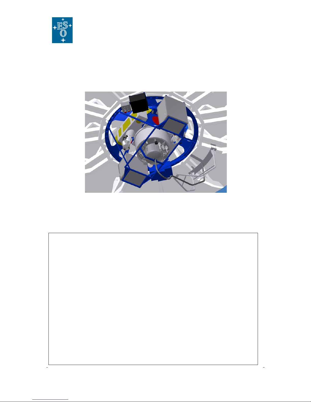
1.Introduction
Figure 1: 3D CAD view of the X-shooter spectrograph at the Cassegrain focus of one of the VLT
Unit Telescope.
Table 1: X-shooter characteristics and observing capabilities
Wavelength range
300-2500 nm split in 3 arms
UV-blue arm
Range: 300-550 nm in 12 orders
Resolution: 5100 (1" slit)
Slit width: 0.5”, 0.8”, 1.0”, 1.3”, 1.6”, 5.0”
Detector: 4k x 2k E2V CCD
Visual-red arm
Range: 550-1000 nm in 14 orders
Resolution: 8800 (0.9" slit)
Slit width: 0.4”, 0.7”, 0.9”, 1.2”, 1.5”, 5.0”
Detector: 4k x 2k MIT/LL CCD
Near-IR arm
Range: 1000-2500 nm in 16 orders
Resolution: 5100 (0.9" slit)
Slit width: 0.4”, 0.6”, 0.9”, 1.2”, 1.5”, 5.0”
Detector: 2k x 1k Hawaii 2RG
Slit length
11”
Beam separation
Two high efficiency dichroics
Atmospheric dispersion compensation
In the UV-Blue and Visual-red arms
Integral field unit
1.8" x 4" reformatted into 0.6" x 12"

X-shooter
User Manual
Doc:
Issue
Date
Page
VLT-MAN-ESO-12000-0115
1
01.03.2009
8 of 60
ESO, Karl-Schwarzschild-Str. 2, 85748 Garching bei München, Germany
1.1 Scope
The X-shooter User Manual provides extensive information on the technical characteristics of
the instrument, its performances, observing and calibration procedures and data reduction.
1.2 X-shooter in a nutshell
X-shooter is a single target spectrograph for the Cassegrain focus of one of the VLT UTs
covering in a single exposure the spectral range from the UV to the K band. The spectral
format is fixed. The instrument is designed to maximize the sensitivity in the spectral range
through the splitting in three arms with optimized optics, coatings, dispersive elements and
detectors. It operates at intermediate resolutions (R=4000-14000, depending on wavelength
and slit width) sufficient to address quantitatively a vast number of astrophysical applications
while working in a background-limited S/N regime in the regions of the spectrum free from
strong atmospheric emission and absorption lines. A 3D CAD view of the instrument
attached to the telescope is shown on Figure 1. Main instrument characteristics are
summarized in Table 1.
X-shooter was built by a Consortium involving institutes from Denmark, Italy, The
Netherlands, France and ESO. Name of the institutes and their respective contributions are
given in Table 2.
1.3 Shortcuts to most relevant facts for proposal preparation
•The fixed spectral format of X-shooter: see Table 9 on page 23
•Spectral resolution as a function of slit width: see Table 10 on page 24
•Information on the IFU: see page 13
•Information on limiting magnitudes in the continuum: see Section 2.3.3 on page 24
•Information on observing modes: see section 3.1 on page 27
•Observing strategy and sky subtraction: see Section 3.3 on page 28
•Overhead computation: see Section 3.4 on page 30
Table 2: collaborating institutes and their contributions
Collaborating institutes
Contribution
Copenhagen University
Observatory
Backbone unit, UVB spectrograph, Mechanical
design and FEA, Control electronics
ESO
Project Management and Systems Engineering,
Detectors, final system integration,
commissioning, logistics
Paris-Meudon Observatory,
Paris VII University
Integral Field Unit, Data Reduction Software
INAF - Observatories of Brera,
Catania, Trieste and Palermo
UVB and VIS spectrograph, Instrument Control
Software, optomechanical design.
Astron, Universities of
Amsterdam and Nijmegen
NIR spectrograph, contribution to Data
Reduction Software

X-shooter
User Manual
Doc:
Issue
Date
Page
VLT-MAN-ESO-12000-0115
1
01.03.2009
9 of 60
ESO, Karl-Schwarzschild-Str. 2, 85748 Garching bei München, Germany
1.4 List of Abbreviations & Acronyms
This document employs several abbreviations and acronyms to refer concisely to an item,
after it has been introduced. The following list is aimed to help the reader in recalling the
extended meaning of each short expression:
A&G
Acquisition and Guiding
DCS
Detector Control Software
DFS
Data Flow System
ESO
European Southern Observatory
GUI
Graphical User Interface
ICS
Instrument Control Software
IFU
Integral Field Unit
ISF
Instrument Summary File
IWS
Instrument Workstation
LCC
LCU Common Software
LCU
Local Control Unit
N/A
Not Applicable
PAE
Preliminary Acceptance Europe
P2PP
Phase 2 Proposal Preparation
TBC
To Be Clarified
QE
Quantum Efficiency
SNR
Signal to Noise Ratio
TBD
To Be Defined
TCS
Telescope Control Software
TSF
Template Signature File
VLT
Very Large Telescope
1.5 Reference Documents
1. X-shooter Calibration plan, v1.0, XSH-PLA-ESO-12000-0088
2. X-shooter Templates Reference Manual, v0.2, XSH-MAN-ITA-8000-0031

X-shooter
User Manual
Doc:
Issue
Date
Page
VLT-MAN-ESO-12000-0115
1
01.03.2009
10 of 60
ESO, Karl-Schwarzschild-Str. 2, 85748 Garching bei München, Germany
2.Technical description of the instrument
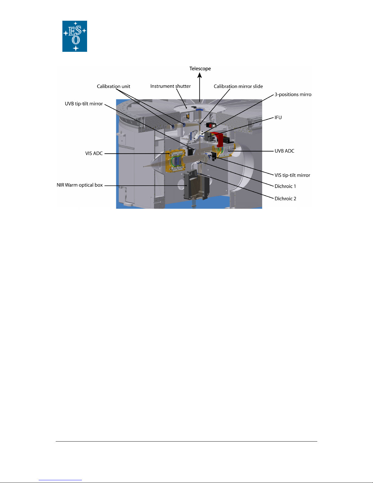
2.1 Overview of the opto-mechanical design
Figure 2 shows a schematic view of the layout of the instrument. It consists of four main
components:
•The backbone which is directly mounted on the Cassegrain derotator of the
telescope. It contains all pre-slit optics: the calibration unit, a slide with the 3-
positions mirror and the IFU, the acquisition and guiding camera, the dichroic box
which splits the light between the three arms, one piezo tip-tilt mirror for each arm to
allow active compensation of backbone flexures, atmospheric dispersion
compensators (ADCs) in the UVB and VIS arms and a warm optical box in the NIR
arm.
Figure 2: Schematic overview of X-shooter

X-shooter
User Manual
Doc:
Issue
Date
Page
VLT-MAN-ESO-12000-0115
1
01.03.2009
11 of 60
ESO, Karl-Schwarzschild-Str. 2, 85748 Garching bei München, Germany
•The three arms are fixed format cross-dispersed échelle spectrographs that operate
in parallel. Each one has its own slit selection device.
oThe UV-Blue spectrograph covers the 300 – 550 nm wavelength range with a
resolving power of 5100 (for a 1” slit)
oThe Visible spectrograph covers the range 550 - 1000 nm with a resolving
power of 7500 (0.9” slit).
oThe near-IR spectrograph: this arm covers the range 1000 - 2500 nm with a
resolving power of 5100 (0.9” slit). It is fully cryogenic.
2.2 Description of the instrument sub-systems
This section describes the different sub-systems of X-shooter in the order they are encountered along
the optical path going from the telescope to the detectors (see
Figure 2). The functionalities of the different sub-units are explained and reference is made
to their measured performance.
2.2.1 The Backbone
The Instrument Shutter and The calibration unit
In the converging beam coming from the telescope, the first element is the telescope
entrance shutter which allows safe daytime use of X-shooter for tests and calibration without
stray-light entering the system from the telescope side.
Then follows the Calibration Unit that allows to select a choice of flat-fielding and wavelength
calibration lamps. This unit consists of a mechanical structure with calibration lamps, an
integrating sphere, relay optics that simulate the f/13.6 telescope beam, and a mirror slide
with 3 positions that can be inserted in the telescope beam:
Figure 3: 3D view of a cut through the backbone.

X-shooter
User Manual
Doc:
Issue
Date
Page
VLT-MAN-ESO-12000-0115
1
01.03.2009
12 of 61
ESO, Karl-Schwarzschild-Str. 2, 85748 Garching bei München, Germany
•one free position for a direct feed from the telescope,
•one mirror which reflects the light from the integrating equipped with:
owavelength calibration Ar, Hg, Ne and Xe Penray lamps operating
simultaneously
othree flatfield halogen lamps equipped with different balancing filters to
optimize the spectral energy distribution for each arm
•one mirror which reflects light from:
oa wavelength calibration hollow cathode Th-Ar lamp
oa D2lamp for flatfielding the bluest part of the UV-Blue spectral range
A more detailed description of the functionalities of the calibration system is given in Section
4.
The Acquisition and Guiding slide.
Light coming either directly from the telescope or from the Calibration Unit described above
reaches first the A&G slide. This structure allows to put into the beam either:
•a flat 45˚ mirror with 3 positions mirror:
oacquisition and imaging: send the full 1.5’×1.5’ field of view to the A&G
camera. This is the position used during all acquisition sequences;
ospectroscopic observations and monitoring: a slot lets the central 10”×15” of
the field go through to the spectrographs while reflecting the peripheral field to
the A&G camera. This is the position used for all science observations.
oartificial star: a 0.5” pinhole used for optical alignment and engineering
purposes;
•the IFU (described below on page 13);
•a 50/50 pellicle beam splitter at 45˚ used look down into the instrument with the A&G
camera and is exclusively used for engineering purposes.

X-shooter
User Manual
Doc:
Issue
Date
Page
VLT-MAN-ESO-12000-0115
1
01.03.2009
13 of 60
ESO, Karl-Schwarzschild-Str. 2, 85748 Garching bei München, Germany
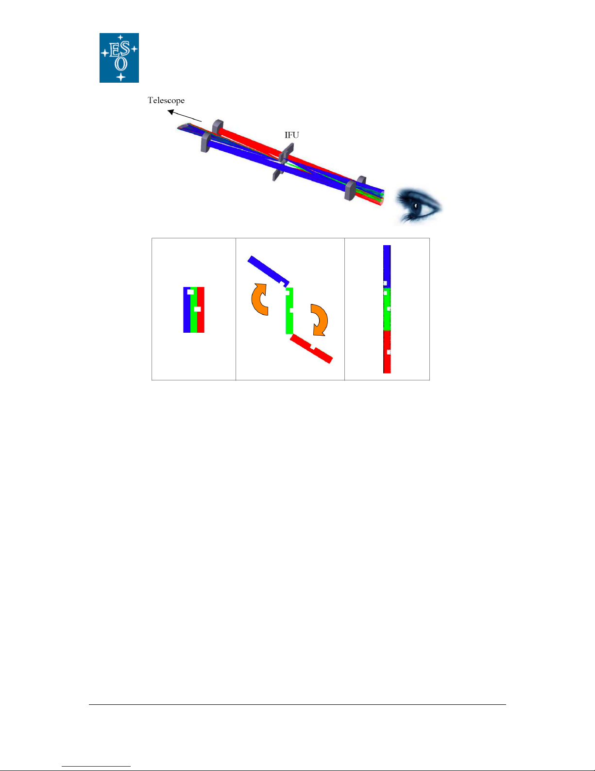
The IFU
The Integral Field Unit is an image slicer that re-images an input fie0d of 4”x1.8” into a
pseudo slit of 12”x0.6”. The light from the central slice is directly transmitted to the
spectrographs. The two lateral sliced fields are reflected toward the two pairs of spherical
mirrors and re-aligned at both ends of the central slice in order to form the exit slit as
illustrated in Figure 4. Due to these four reflections the throughput of the two lateral fields is
reduced with respect to the directly transmitted central one. The measured overall efficiency
of the two lateral slitlets is ~85% of the direct transmission (TBC) but drops to ~50% (TBC)
below 400 nm due to reduced coating efficiency in the blue.
The Acquisition and Guiding Camera
The A&G camera allows to visually detect and centroid objects from the U- to the z-band.
This unit consists in:
•a filter wheel equipped with a full UBVRI Johnson filter set and a full Sloan Digital
Sky Survey (SDDS) filter set. Transmission curves are provided in appendix 5.4.
Figure 4: Top: view of the effect of the IFU. The central field is directly transmitted to
form the central slitlet (green) while the each lateral field (in blue and red) are reflected
toward a pair of spherical mirrors and realigned at the end of the central slice to form
the exit slit. Bottom: The field before (left) and after the IFU (right). The IFU acts such
that the lateral fields seems to rotate around a corner of their small edge. The two
white slots are not real gaps but just guides to help visualize the top and the bottom of
each slice in the drawing.

X-shooter
User Manual
Doc:
Issue
Date
Page
VLT-MAN-ESO-12000-0115
1
01.03.2009
14 of 60
ESO, Karl-Schwarzschild-Str. 2, 85748 Garching bei München, Germany
•a Peletier cooled, 13 µm pixel, 512×512 E2V broad band coated Technical CCD57-
10 onto which the focal plane is re-imaged at f/1.91 through a focal reducer. This
setup provides a plate scale of 0.173”/pix and a field of view of 1.47’×1.47’. The QE
curve of the detector is provided in appendix 5.3.
This acquisition device –that can also be used to record images of the target field through
different filters– provides a good enough sampling to centroid targets to <0.1” accuracy in all
seeing conditions and reaches limiting magnitudes given in columns 4 and 5 of Table 3.
Table 3: The overall transmission in UBVRI (column 3) along with effective central wavelength and
FWHM (columns 1 and 2) of the A&G Camera UBVRI filters. Limiting magnitudes to a SNR of 5 and
10 reached in 3s integration are given in column 4 and 5. These were computed over an area
containing 80% of the energy for a seeing of 0.8”, for airmass 1, with sky brightness 3 days from new
moon.
Filter
[1]
Effective
Central λ
[2]
Effective
FWHM
[3]
Efficiency incl.
atmosphere
[4]
Limiting Mag.
(3s, SNR=5)
[5]
Limiting Mag.
(3s, SNR=10)
U
370 nm
39 nm
10%
21.1
20.2
B
441 nm
100 nm
17%
23.1
22.2
V
535 nm
80 nm
27%
22.8
21.9
R
639 nm
116 nm
21%
22.4
21.5
I
829 nm
175 nm
16%
21.9
21.0
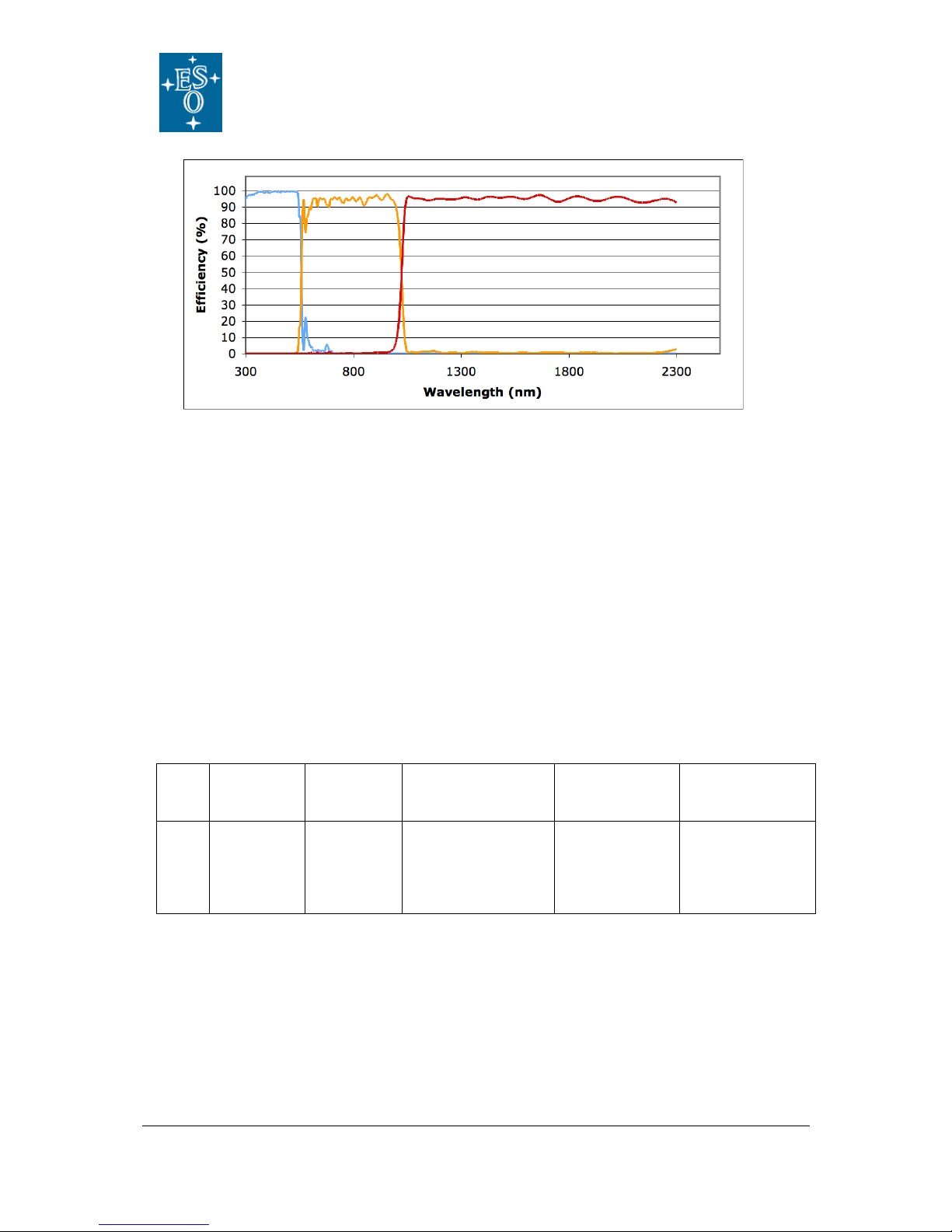
The dichroic box
Light is split and distributed to the three arms by two highly efficient dichroic beam splitters.
These are the first optical elements encountered by the science light. The first dichroic at an
incidence angle of 15˚ reflects more than 98% of the light between 350 and 543 nm and
transmits ~95% of the light between 600 and 2300 nm. The second dichroic, also at 15˚
incidence, has a reflectivity above 98% between 535 nm and 985 nm and transmits more
than 96% of the light between 1045 and 2300 nm. The combined efficiency of the two
dichroics is shown in Figure 5: it is well above 90% over most of the spectral range.
Figure 5: The combined efficiency of the two dichroic beam splitters. In blue: reflection
on dichroic 1; in orange: transmission through dichroic 1 and reflection on dichroic 2; in
red: transmission through dichroics 1 & 2.

X-shooter
User Manual
Doc:
Issue
Date
Page
VLT-MAN-ESO-12000-0115
1
01.03.2009
15 of 60
ESO, Karl-Schwarzschild-Str. 2, 85748 Garching bei München, Germany
The flexure compensation tip-tilt mirrors
Light reflected and/or transmitted by the two dichroics reaches, in each arm, a folding mirror
mounted on piezo tip-tilt mount. These mirrors are used to fold the beam and correct for
backbone flexure to keep the relative alignment of the three spectrograph slits within less
than 0.02” at any position of the instrument. They also compensate for shifts due to
atmospheric differential refraction between the telescope tracking wavelength (fixed at 470
nm for all X-shooter observations) and the undeviated wavelength of the two ADCs (for UVB
and VIS arms) and the middle of the atmospheric dispersion range for the NIR arm.
The Focal Reducer and Atmospheric Dispersion Correctors
Both UVB and VIS pre-slit arms contain a focal reducer and an ADC. These focal reducer-
ADCs consist of two doublets cemented onto two counter rotating double prisms. The focal
reducers bring the focal ratio from f/13.41 to ~f/6.5 and provide a measured plate scale at the
entrance slit of the spectrographs of 3.91”/mm in the UVB and 3.82”/mm in the VIS. The
ADCs compensate for atmospheric dispersion in order to minimize slit losses and allow
orienting the slit to any position angle on the sky up to a zenith distance of 60˚. The zero-
deviation wavelengths are 405 and 633 nm for the UVB and the VIS ADCs respectively. In
the AUTO mode, their position is updated every 60s based on information taken from the
telescope database.
The NIR arm is not equipped with an ADC. The NIR arm tip-tilt mirror compensates for
atmospheric refraction between the telescope tracking wavelength (470 nm) and 1310 nm
which corresponds to the middle of the atmospheric dispersion range for the NIR arm. This
means that this wavelength is kept at the center of the NIR slit. At a zenithal distance of 60°
the length of the spectrum dispersed by the atmosphere is 0.35”, so the extremes of the
spectrum can be displaced with respect to the center of the slit by up to 0.175”. If
measurement of absolute flux is an important issue, the slit should then be placed at
parallactic angle.

X-shooter
User Manual
Doc:
Issue
Date
Page
VLT-MAN-ESO-12000-0115
1
01.03.2009
16 of 60
ESO, Karl-Schwarzschild-Str. 2, 85748 Garching bei München, Germany
2.2.2 The UVB spectrograph
Slit carriage
The first opto-mechanical element of the spectrograph is the slit carriage. Besides the slit
selection mechanism, this unit consists of a field lens placed just in front of the slit to reimage
the telescope pupil onto the spectrograph grating, and the spectrograph shutter just after the
slit. The slit mask is a laser cut Invar plate manufactured with the LPKF Laser Cutter used for
FORS and VIMOS. It is mounted on a motorized slide in order to select one of the 9 positions
available. All science observation slits are 11” high and different widths from 0.5” to 5” (the
latter for spectro-photometric calibration) are offered. In addition a single pinhole for spectral
format check and order tracing and a 9-pinhole mask for wavelength calibration and spatial
scale mapping are available (see Table 4).
Table 4: UVB spectrograph slits and calibration masks
Size
Purpose
0.5”×11” slit
SCI / CAL
0.8”×11” slit
SCI / CAL
1.0”×11” slit
SCI / CAL
1.3”×11” slit
SCI / CAL
1.6”×11” slit
SCI / CAL
5.0”×11” slit
CAL
Raw of 9 pinholes of 0.5”
∅spaced at 1.4”
CAL
0.5” ∅pinhole
CAL
Figure 6: The UVB spectrograph optical layout

X-shooter
User Manual
Doc:
Issue
Date
Page
VLT-MAN-ESO-12000-0115
1
01.03.2009
17 of 60
ESO, Karl-Schwarzschild-Str. 2, 85748 Garching bei München, Germany
Optical layout
The optical layout of the UVB spectrograph is presented in Figure 6. Light from the entrance
slit, placed behind the plane of the figure, feeds a 5˚ off-axis Maksutov-type collimator
through a folding mirror. The collimator consists of a spherical mirror and a diverging fused
silica corrector lens with only spherical surfaces. The collimated beam passes through a 60˚
silica prism twice to gain enough cross-dispersion. Main dispersion is achieved through a
180 grooves/mm échelle grating blazed at 41.77˚. The off-blaze angle is 0.0˚, while the off-
plane angle is 2.2˚. After dispersion, the collimator creates an intermediate spectrum near
the entrance slit, where a second folding mirror has been placed. This folding mirror acts also
as field mirror. Then a dioptric camera (4 lens groups with CaF2 or silica lenses, 1 aspherical
surface) reimages the cross-dispersed spectrum at f/2.7 (plate scale 9.31”/mm) onto a
detector that is slightly tilted to compensate for a variation of best focus with wavelength. The
back focal length is rather sensitive to temperature changes. It varies by ~22.7µm/˚C which
corresponds to a defocus of 9µm/˚C or ~0.08”/˚C. This is automatically compensated at the
beginning of every exposure by moving the triplet+doublet of the camera by -10.9µm/˚C.
Detector
The UVB detector is a 2048×4102, 15µm pixel CCD from E2V (type CCD44-82) of which
only a 1800×3000 pixels window is used. The CCD cryostat is attached to the camera with
the last optical element acting as a window. The operating temperature is 153K. The CCD
control system is a standard ESO FIERA controller shared with the VIS CCD. The list of
readout modes offered for science observations is given in Table 5.
One more readout mode (1000×1000 window, low gain, fast readout, 1x1 binning)
exclusively used for flexure measurement and engineering purposes is also implemented.
Measured properties and performances of this system are summarized in Table 6. The
associated shutter, located just after the slit is a 25mm bi-stable (2 coil, zero dissipation)
shutter from Uniblitz (type BDS 25). Full transit time is 13ms. Since the slit is 2.8mm high
(11” at f/6.5), the illumination of the detector is homogenous within <<10ms.
Table 5: List of detector readout modes offered for science observations
Readout mode
Gain [e-/ADU]
Speed
Binning
name
UVB
VIS
[kpix/s]
Spatial dir.
Dispersion dir.
100k/1pt/hg
1
1
100k/1pt/hg/1x2
1
2
100k/1pt/hg/2x2
High
[0.67]
High
[0.64]
Slow
[100]
2
2
400k/1pt/lg
1
1
400k/1pt/lg/1x2
1
2
400k/1pt/lg/2x2
Low
[1.75]
Low
[1.5]
Fast
[400]
2
2

X-shooter
User Manual
Doc:
Issue
Date
Page
VLT-MAN-ESO-12000-0115
1
01.03.2009
18 of 60
ESO, Karl-Schwarzschild-Str. 2, 85748 Garching bei München, Germany
UVB
VIS
NIR
Detector type
E2V CCD44-82
MIT/LL CCID 20
substrate
removed Hawaii
2RG
Operating
temperature
153 K
135 K
81 K
QE
80% at 320 nm
88% at 400 nm
83% at 500 nm
81% at 540 nm
78% at 550 nm
91% at 700 nm
74% at 900 nm
23% at 1000 nm
85%
Number of
pixels
2048×3000
(2048×4102 used in
windowed readout)
2048×4096
2048×2048
(1024×2048
used)
Pixel size
15 µm
15µm
18µm
Gain
(e-/ADU)
High: 0.67
Low: 1.75
High: 0.64
Low: 1.5
2.12
Readout noise
(e- rms)
Slow: 2.6
Fast: 4.5
Slow: 3.2
Fast: 5.3
Short DIT: 22
DIT=600s: 5.5
Saturation
(ADU)
65000 (TBC)
65000
45000 (TBC)
Full frame
readout time
(s)
1x1, slow-fast: 70-19
1x2, slow-fast: 38-12
2x2, slow-fast: 22-8
1x1, slow-fast: 92-24
1x2, slow-fast: 48-14
2x2, slow-fast: 27-9
0.88 (for single
readout, TBC)
Dark current
level
<0.2e-/pix/h (TBC)
<1.1e-/pix/h (TBC)
14 e-/pix/h
(TBC)
Fringing
amplitude
-
~5% peak-to-valley
-
Non-lineariy
<0.7%
<0.8%
<1% up to
45000 ADUs
(TBC)
Readout
direction
Main disp. dir.
Main disp. dir.
-
Prescan and
overscan areas
1x1 and 1x2: X=1-48
and 2097-2144
2x2: X=1-24 and 1049-
1072
1x1 and 1x2: pix 39-48
and 2097-2144
2x2: 19-24 and 1049-
1072
-
Flatness
<8µm peak-to-valley
Table 6: measured properties of the X-shooter detectors

X-shooter
User Manual
Doc:
Issue
Date
Page
VLT-MAN-ESO-12000-0115
1
01.03.2009
19 of 60
ESO, Karl-Schwarzschild-Str. 2, 85748 Garching bei München, Germany
2.2.3 The VIS spectrograph
Slit carriage
The slit carriage of the VIS spectrograph is identical to that of the UVB but the available slits
are different. All the science observation slits are 11” high and different widths are offered
from 0.4” to 5” (see Table 7).
Table 7: VIS spectrograph slits and calibration masks
Size
Purpose
0.4”×11” slit
SCI / CAL
0.7”×11” slit
SCI / CAL
0.9”×11” slit
SCI / CAL
1.2”×11” slit
SCI / CAL
1.5”×11” slit
SCI / CAL
5.0”×11” slit
CAL
Raw of 9 pinholes of 0.5”
∅spaced at 1.4”
CAL
0.5” ∅pinhole
CAL
Optical layout
The optical layout of the VIS spectrograph is very similar to that of the UVB (see Figure 6).
The collimator (mirror+corrector lens) is identical. For cross-dispersion, it uses a 49˚ Schott
SF6 prism in double pass. The main dispersion is achieved through a 99.4 grooves/mm,
54.0˚ blaze échelle grating. The off-blaze angle is 0.0˚ and the off-plane angle is 2.0˚. The
camera (3 lens groups, 1 aspherical surface) reimages the cross-dispersed spectrum at f/2.8
(plate scale 8.98”/mm) onto the detector (not tilted). Focussing is obtained by acting on the
triplet+doublet sub-unit of the camera. However, unlike the UVB arm, the back focal length
varies less than 1µm/˚C (image blur <0.004”/˚C) hence no thermal focus compensation is
needed.
Detector
The VIS detector is 2048×4096, 15µm pixel CCD from MIT/LL (type CCID-20). Like for the
UVB arm, the cryostat is attached to the camera with the last optical element acting as a
window. The operating temperature is 135K. It shares its controller with the UVB detector
and the same readout modes are available (see Table 5). Measured properties and
performances are given in Table 6. The shutter system is identical to the UVB one.
2.2.4 The NIR spectrograph
The NIR spectrograph is fully cryogenic. It is cooled with a liquid nitrogen bath cryostat and
operates at 105 K.
Pre-slit optics and entrance window
After the dichroic box and two warm mirrors M1 (cylindrical) and M2 (spherical, mounted on a
tip-tilt stage and used for flexure compensation, see description on p. 15) light enters the
cryostat via the Infrasil vacuum window. To avoid ghosts, this window is tilted 3 degrees
about the Y-axis. After the window, light passes the cold stop, and is directed towards the
entrance slit via two folding mirrors M3 (flat) and M4 (spherical).

X-shooter
User Manual
Doc:
Issue
Date
Page
VLT-MAN-ESO-12000-0115
1
01.03.2009
20 of 60
ESO, Karl-Schwarzschild-Str. 2, 85748 Garching bei München, Germany
Slit wheel
A circular laser cut Invar slit mask is pressed in between two stainless steel disks with 12
openings forming the wheel. The wheel is positioned by indents on the circumference of the
wheel with a roll clicking into the indents. All the science observation slits are 11” high and
different widths are offered from 0.4” to 5” (see Table 8).
Table 8: NIR spectrograph slits and calibration masks
Size
Purpose
0.4”×11” slit
SCI / CAL
0.6”×11” slit
SCI / CAL
0.9”×11” slit
SCI / CAL
1.2”×11” slit
SCI / CAL
1.5”×11” slit
SCI/CAL
5.0”×11” slit
CAL
Raw of 9 pinholes of 0.5”
∅spaced at 1.4”
CAL
0.5” ∅pinhole
CAL
Optical layout
The optical layout of the NIR spectrograph is presented in Figure 7. The conceptual design is
the same than for the UVB and the VIS spectrographs. Light entering the spectrograph via
the entrance slit and folding mirror M5 feeds an off-axis Maksutov-inspired collimator. In this
case, the collimator is made of 2 spherical mirrors M6 and M7 plus an Infrasil corrector lens
(with only spherical surfaces). In order to get enough cross dispersion, three prisms are used
Figure 7: The NIR spectrograph optical layout.