DORIC Fiber Photometry System User manual

Fiber Photometry System
Getting Started Guide
Version 2.2.1

Contents
1 Fiber Photometry Systems at a Glance 3
1.1 Systems Overview .................................................... 3
1.2 Fiber Photometry Console ............................................... 5
1.3 Integrated Connectorized Fluorescence Mini Cube ................................ 6
1.4 Light Sources ....................................................... 7
1.5 Rotary Joints ....................................................... 10
1.6 Low Autofluorescence Patch Cords .......................................... 10
1.7 Photodetectors ..................................................... 11
2 Getting Started 14
2.1 Connecting the Fiber Photometry System ...................................... 14
2.2 Configuring the Fiber Photometry Console ..................................... 17
2.3 Using the Fiber Photometry Analysis Module .................................... 25
3 Support 26
3.1 Contact us ........................................................ 26
2

1
Fiber Photometry Systems at a Glance
1.1 Systems Overview
In neuroscience, Fiber photometry denotes a method whereby chronically implanted optical fibers deliver excitation
light to neurons tagged with a fluorescent calcium indicator and collect their overall activity-induced fluorescence. Fiber
photometry sums up the activity-induced fluorescence of all neurons expressing the indicator(s).
In addition to systems custom-designed for your needs, we offer systems for typical modular fiber photometry mea-
surement setups. The Locked-in or Sequential Detection for GCaMP Isosbestic and Functional Excitations system measures
the 405 nm (isosbestic point) excited GCaMP fluorescence, and the 465 nm excited calcium-dependent GCaMP fluo-
rescence, on a single photodetector. The Separated Two Fluorophores Fluorescence contains all the items necessary to
perform photometry measurements of two independent colors in freely-moving animals for GFP-like and RFP-like fluo-
rophores.
A typical set-up for freely behaving animals contains of the following elements (Fig. 1.1).
• A Fiber photometry console to synchronize output control and the acquisition of data.
• An Integrated fluorescence mini cube where beam splitters combine the excitation wavelengths and separate the
emission wavelengths. This Fluorescence Mini Cube comes with the following.
–One or more Built-in fluorescence detector heads capable of sensing low-intensity light. The fluorescence emis-
sion can be collected with one photodetector and subsequently demodulated or, after spectral separation,
collected with respective photodetectors.
–One or more Built-in LED optical heads that provide light for the experiment.
• An optional Fiber-optic rotary joint can be used to allow free movement of the experimental subject.
• An Optical cannula, with connecting Fiber-optic patch cords, to deliver light to the subject.
• A Low Autofluorescence Patch Cord to allow light collection with minimal fluorescence noise.
The following section describes these standard elements and their purpose.
Chapter 1. Fiber Photometry Systems at a Glance 3

ilFMC.jpg
Figure 1.1: Typical Modular Fiber Photometry Measurement Setup
Chapter 1. Fiber Photometry Systems at a Glance 4

1.2 Fiber Photometry Console
This FPGA based data acquisition unit synchronizes the output control and the acquisition of the input data. This device
seamlessly integrates with Doric Neuroscience Studio software, which provides the user-interface for multi-channel
photometry experiments.
The software interface enables control over the CW excitation light pulses, square or sinusoidal waveform of an ex-
ternal source (i.e. LED driver) with 4 digital input/outputs and 4 analog voltage outputs. The software interface displays
real-time data of up to 4 detectors input signals and performs data acquisition. The other new functionalities are being
developed and users can upload them as they become available.
The Fiber Photometry Console inputs and outputs are shown in figures 1.2 and 1.3.
Figure 1.2: Front view of the Fiber Photometry Console: Inputs and outputs
• The LCD Screen displays console information.
• The Digital/IO ports sends 0-4.75 V TTL pulses.
• The HDMI port acquires digital signals and digital communication SPI and LVDS via a custom pinout HDMI con-
nector.
• The Analog-out ports send a variable ±4.75 V analog signal signal.
• The Analog-in ports acquire analog signals up to ±10 V.
• The Power On/Off opens and closes the device.
Chapter 1. Fiber Photometry Systems at a Glance 5

Figure 1.3: Back view: Maintenance and Power Supply
• The 12V port connects to the 12 VDC Power supply.
• The USB port allows a USB-B connection to a computer.
• The Service port is a USB-B port through which the firmware of the device can be updated.
• The USB-3 charging port is currently disabled.
1.3 Integrated Connectorized Fluorescence Mini Cube
Figure 1.4: 4-port Fluorescence Mini Cube
The integrated Fluorescence Mini Cube is an optical assembly that allows the combination of multiple excitation and detec-
tion signals. The cubes are classified by their number of ports, with 3, 4, 5, 6 and 7 port cubes available. The ports are
each classified according to their usage, and are also qualified by a wavelength band corresponding to the bandwidth of
optical filters within the cube.
•Eand IE (Fig. 1.4) represent entry ports for fluorescence and isosbestic point excitation light. Each port of this type
comes with a Built-in LED Optical Head that contains the following elements.
–The Intensity Adjustment Ring (Fig. 1.5a) allows additional adjustment of the overall output intensity of
light.
–The M8 connector port (Fig. 1.5a) is used to connect the optical head to the LED Driver using a Male-Female
M8 Cable.
Chapter 1. Fiber Photometry Systems at a Glance 6

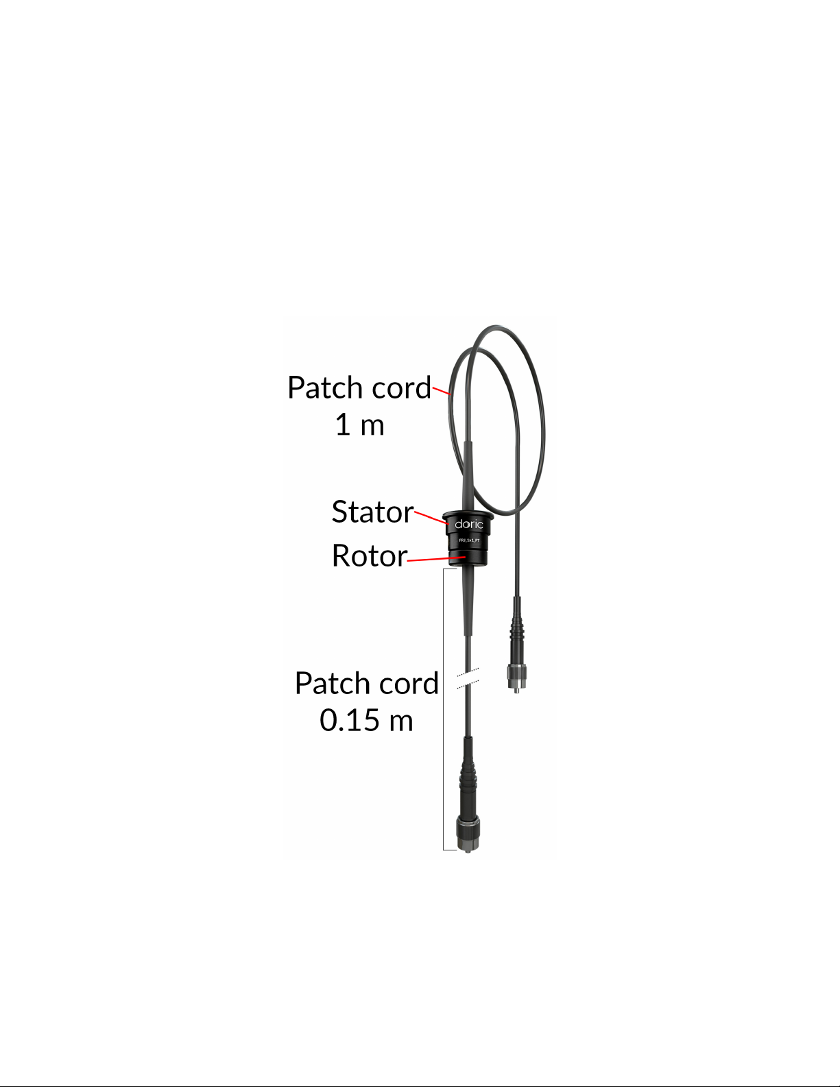
–The Heat-sink Fins (Fig. 1.5a) are used to evacuate heat from the light source, allowing stable output power.
Ensure the fins are not blocked to allow proper cooling.
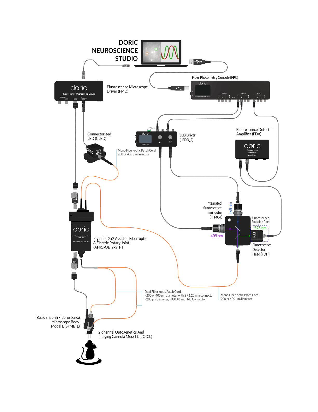
•F(Fig. 1.4) represents ports for fluorescence emission light. Each port of this type comes with a Built-in Doric
Fluorescence Detector Head.
–The M5 Connector (Fig. 1.5b) allows the Fluorescence Detector Head to be connected to the Fluorescence
Detector Amplifier using an M5 male/male connection cable.
–For extremely low light level applications, the fluorescence ports (F, F1, etc.) can have a Built-in Photomultiplier
Tube rather than a Built-in Fluorescence Detector Head.
•O(Fig. 1.4) represents optogenetic activation or silencing ports. These are always FC receptacles to allow connec-
tion to laser or fluorescence light sources.
•S(Fig. 1.4) represents the exit port to the sample. These are always FC receptacles to allow connection to an ex-
perimental subject.
(a) Built-in LED Optical Head (b) Built-in Fluorescence Detector Head
Figure 1.5: ilFMC Built-in components
1.4 Light Sources
1.4.1 LED Driver
Doric LED Drivers can be used as a stand-alone device or controlled via USB port. Each channel connects to a single
Connectorized LED which can be controlled manually or via the Doric Neuroscience Studio Software.
The LEDs drivers can be used as a stand alone device. During stand-alone operation, it is possible to change the operating
mode (CW or external analog mode) and the current sent to the Connectorized LED. These changes can be done directly
on the device with the control knobs and the LCD display.
Connecting the LED drivers to a computer provides the user with more options. Doric Neuroscience Studio Software
allows the access to more operating modes like CW, external TTL, external analog, internal TTL and internal Complex
modes. Doric Neuroscience Studio Software enables the creation of different sequences of light source activation. It
also provides the possibility to let these sequences be triggered or paused by an external signal. If more power is needed,
it is possible to overdrive the LED driver with the software. Our LED driver has a live pulse capability allowing the
visualization of the signal modulation on the input BNC in a scope-like manner.
• The LCD display (Fig. 1.7) allows easy operation and monitoring. For each channel, the LCD displays the type of
light source (LED), the operating mode, the center wavelength in nm and the current setting.
Chapter 1. Fiber Photometry Systems at a Glance 7

Figure 1.6: LED Drivers; 1-, 2- and 4-channel
Figure 1.7: Front view of a 4-channel LED Driver
• The Power key must be properly inserted into the key switch to enable operation of the light source(s) connected
to the driver. Note that, despite its similar shape, the power key is not a standard micro SD card such as those used
in some digital cameras. Do not attach the Key to a key fob or similar holder; this may prevent proper insertion of
the Power key.
• The M8 connector is used to link the driver and LED.
• The Interlock Connector Plug (Fig. 1.8) allows the user to connect the driver to an interlock system. It is recom-
mended to connect the interlock plug to a laboratory interlock system. This is critical when using LEDs in the UV
or Infrared spectrum, as they are invisible to the naked eye.
• The Input BNC allows the control of the LED driving current of the corresponding source with an analog or TTL
signal.
• The Output BNC are used to monitor the driving current of the corresponding light source.
• The 12 VDC power input connects the driver to its 12 VDC power supply.
• The USB-B Connector allows the driver to be connected to a computer using a USB-A/USB-B cable.
Chapter 1. Fiber Photometry Systems at a Glance 8

Figure 1.8: Rear view of a 4-channel LED Driver
• The On/Off switch (Fig. 1.9) turns on/off the driver.
Figure 1.9: Side view of a 4-channel LED Driver
Chapter 1. Fiber Photometry Systems at a Glance 9

1.5 Rotary Joints
The various cables and fibers used to connect a Fiber Photometry system to an animal can be problematic when used
with a freely-moving animal subject. Rigid cables can limit animal freedom and comfort, while excessive torque applied
to the cables by animal movement can break them. A rotary joint allows the cables and fibers to move with the animal,
without effect on signal quality. When used for fiber photometry, Pigtailed Rotary Joints are favored.
1.5.1 Pigtailed 1x1 Fiber-optic Rotary Joint
The pigtailed variant of the 1x1 Fiber-optic Rotary Joint (Fig. 1.10) includes FC connectorized fiber-optic patch cords
pigtailed on both sides of the rotary joint. This involves pre-alignment of the optical fibers, which reduces intensity
variation in rotation normally observed. They have been designed for applications where optical power variation must
be minimized, such as fiber photometry. These rotary joints are optimized for use with 400 µm and 200 µm diameter
core optical fibers, with an NA of 0.57.
Figure 1.10: Pigtailed 1x1 Fiber-optic Rotary Joint
1.6 Low Autofluorescence Patch Cords
All optical fibers posses a certain innate fluorescence due to their chemical composition. Often called Autofluorescence,
this light can interfere in photometry measurements by overwhelming them. The Doric Lenses Low Autofluorescence (LAF)
Patch Cords have minimal autofluorescence and are thus ideal for fiber photometry. All LAF patch cords are identified by
the red Coupling Nut on the connector.
Chapter 1. Fiber Photometry Systems at a Glance 10

1.7 Photodetectors
1.7.1 Doric Fluorescence Detector
The Doric Fluorescence Detector is the first picowatt range sensor developed for fiber photometry. The detector is
directly integrated into our line of ilFMC photometry cubes, though it can be used separately. As the Fluorescence Detec-
tor Head is already described alongside the Integrated Fluorescence Mini Cube, only the Fluorescence Detector Amplifier is
described here.
Fluorescence Detector Amplifier
The Fluorescence Detector Amplifier amplifies the signal coming from the detector head and transmits it to a recording
system using a BNC output. It contains the following elements.
Figure 1.11: Doric Fluorescence Detector Amplifier Elements
• The FDH Connector (Fig. 1.11) is an M5 type connector used to link the amplifier and the head using a shielded
M5 cable.
• The V out Connector (Fig. 1.11) is a BNC type connector used to connect the fluorescence detector with a DAQ
system.
• The Power Indicator light (Fig. 1.11) shines green when the detector is on.
• The Amplifier Mode switch (Fig. 1.11) is used to switch the detection mode from Off to AC or DC.
• The Amplification Level switch (Fig. 1.11) allows the choice of amplification levels at 1, 10 or 100 times.
• The Power Supply connector, located on the back of the unit, is used to connect the 12 V power supply to the
amplifier.
Chapter 1. Fiber Photometry Systems at a Glance 11

1.7.2 Newport Visible Femtowatt Photoreceiver Module Model 2151
This battery-operated photodetector has high gain and detects CW light signals in the picowatt range. When used in
conjunction with a modulated light source and a lock-in amplifier, it achieves sensitivity levels in the femtowatt range.
For this Newport product Doric offers an add-on Fiber-optic adapter that improves coupling efficiency between the large
core, high NA optical fibers used in fiber photometry and the relatively small detector area. Its output analog voltage (-3
to 7.5 V) can be monitored with the Fiber photometry console or any other analog data acquisition box.
For additional details about this device, see the Newport website.
Figure 1.12: Newport Visible Femtowatt Photoreceiver Module Model 2151 + Doric FC Adapter
1.7.3 Hamamatsu H10722-20 Photosensor Module
Warning: The Hamamatsu H10722-20 Photosensor Module is highly sensitive and can be easily damaged if exposed
to high optical power.
For low light level applications that require higher bandwidth, the fluorescence port can be replaced by the photomul-
tiplier tube directly attached to the mini-cube. The Hamamatsu H10722-20 Photosensor Module is compatible with our
cubes and is the most sensitive detector we offer for very low light level detection. Unlike other ports of our mini cubes
that have receptacles and focusing lens, the port for this sensor has a lens that adjusts the beam size to fit the size of
photomultiplier tube (PMT) instead of a receptacle. The PMT is highly sensitive and can be easily damaged if exposed to
high optical power.
For more information about the product, go to the Hamamatsu website.
Chapter 1. Fiber Photometry Systems at a Glance 12

Figure 1.13: Hamamatsu H10722-20 Photosensor Module + Doric FC Adapter
1.7.4 Power Supply for PMT Module C10709
(a) Front view (b) Back view
Figure 1.14: Power Supply for PMT Module C10709
The photosensor module requires a power supply and the C10709 model is recommended. Both drive voltages and
control voltages can be supplied from this single unit.
For more information about this device, go to the Hamamatsu website.
Chapter 1. Fiber Photometry Systems at a Glance 13

2
Getting Started
2.1 Connecting the Fiber Photometry System
Figure 2.1: Connections to the Fiber Photometry Console
Follow this quick start procedure to install and connect the system. We recommend the following order to avoid de-
vice and driver detection problems. If you need more information about each device or the software, refer to the User
Manual of each device.
1. Install the Doric Neuroscience Studio software. Follow the on-screen instructions to install the Doric Neuro-
science Studio on the hard drive of your computer. For more details, refer to the Doric Neuroscience Studio Soft-
ware Manual.
14

2. Connect the Fiber Photometry Console. The console unit is operated with a 12 VDC power supply adapter.
When it is powered, turn on the switch, then connect the console to the computer via a USB cable. A Windows
USB driver will be automatically installed. Open the software to complete the installation of other devices.
3. Connect the Programmable LED Driver. Connect the LED Driver to the power outlet with the included 12 V
AC-DC adapter. When the LED is controlled by the console, light stimulation can be synchronized with the data
acquisition.
• Digital outputs can activate the light source driver with TTL pulses (0 - 5 V square pulses). Connect the LED
Driver Input ports to the Digital I/O. Turn the LED driver switch ON and click on the knob twice for the Ext.
TTL mode. Set a maximal current value corresponding to the excitation power required for the experiment.
• Analog outputs can activate the light source driver with analog pulse sequence. Connect the LED Driver Input
ports to the Analog Out ports. Turn the LED driver switch ON and click on the knob thrice for the MOD mode
(For the LEDD) or ANALOG mode (for the LEDRV). Here, the maximal current value acts as a current ceiling,
meaning even analog signals which would normally provide a higher current will be clipped.
4. Connect the LED Module. The Built-in LED Optical Heads come pre-installed on the Integrated Fluorescence Mini
Cube. Connect the LED Driver to the Built-in LED Optical Heads using the M8 Cables (Fig. 2.1).
Figure 2.2: Integrated Fluorescence Mini-cube Connections
5. Connect the Fluorescence Mini Cube. The sample ports send light to the experimental subject through a LAF
Patch Cord (Fig. 2.2). Please note that the use of a rotary joint may cause some signal variations and loss of light. In
this case, extra care is required during the data analysis and a reference channel is helpful. Perform the following
steps to connect the patch cord to the sample port.
a) Clean the optical fiber connector before insertion. Use isopropanol and a lint-free wipe.
b) With an FC connector, the connector key must be oriented to enter within the receptacle slot to ensure
proper connection (Fig. 2.3).
Chapter 2. Getting Started 15

Figure 2.3: FC connector, Fiber Installation
To reduce the risk of eye injury, it is sound practice to NOT CONNECT/DISCONNECT OPTICAL
FIBERS when the light source is turned on.
6. Connect the Photodetectors.
• The Built-in Fluorescence Detector Head comes pre-installed into the Integrated Fluorescence Mini-Cube. Con-
nect the head to the Fluorescence Detector Amplifier (Fig. 1.11) using the M5 Detector Cable1. Use a BNC cable
to connect the amplifier to the analog input port of the Fiber Photometry Console (Fig. 2.1). We recommend
the verification of gain settings, as signals may vary from one experiment to another and can require different
parameters. In fiber photometry, the DC amplifier mode is needed. The amplification level can be adjusted
depending on the experiment.
• The Newport Visible Femtowatt Photoreceiver Module Model 2151 (Fig. 1.12)is connected to the Fluo-
rescence Mini Cube emission ports with a 600 µm core, NA 0.48 optical fiber patch cord (Fig. 2.2). Use a BNC
cable to connect the Newport photoreceiver module in the Analog input port of the Fiber Photometry con-
sole (Fig. 2.1). The Newport photoreceiver module is battery operated and is turned on with the red switch.
Ensure the module is switched off when the experiment is over to preserve battery power. We recommend
the verification of gain settings, as signals may vary from one experiment to another and can require different
parameters. In any case, the DC low gain setting should be used.
• The Hamamatsu H10722-20 Photosensor Module is linked to the Fluorescence mini cube emission port by
an optical fiber or directly installed on the FMC emission port by an FC connection. The BNC cable of the
photosensor module can be plugged to a power meter to measure the detection signal. The photomultiplier
tube (PMT) is highly sensitive and can be easily damaged if exposed to high optical power.
The Hamamatsu H10722-20 Photosensor Module requires a Power Supply Hamamatsu Model C10709.
On the back of the Photosensor Module, 5 wires of different colors are used to supply operation voltage and
control gain. Each colored wire should be connected to the connector of the same color on the power supply
(Fig. 1.13).
1See the application note if there is difficulty installing the M5 connector
Chapter 2. Getting Started 16

2.2 Configuring the Fiber Photometry Console
To configure the Fiber photometry console, use the Doric Neuroscience Studio. The software allows for the selection of
acquisition modes and parameters. Data acquistion parameters are set on Analog input channels, while the illumination
parameters are set on Digital or Analog outputs, depending on the output signal required. In every mode, the LIVE
button starts all programmed sequences. We recommend the activation of the AUTOSCROLL option that follows the
trace over a given length of time. The length of the displayed trace can be changed. As the LIVE mode keeps up to only a
small amount of data in memory, it is not recommended to use this mode for important data.
To automatically save data, use the RECORD button. This button activates a measurement mode that periodically saves
the data to the hard drive, allowing longer acquisition sessions. To specify the location where data is saved, as well
as which traces are saved, use the Saving options button to open the Saving options window. In this mode it is also
possible to decimate the results, reducing the amount of data points saved and the size of the saved files.
2.2.1 Setting up Continuous acquisition mode
Data acquisition
On an Analog input channel, change the channel mode to Linear. Select an Acquisition Rate from 0.3 to 12 kS/s, de-
pending on the temporal resolution desired. Keep in mind that a higher sampling rate will produce bigger files. For
standard calcium activity measurements, the lowest sampling rate (0.3 kS/s) will give the best signal-to-noise ratio. It is
mandatory to set the photodetector in DC mode for continuous signal acquisition.
Light excitation
When using Digital outputs , set the channel in Continuous Wave (CW) mode. In this configuration, the Digital output
will be 5 V when enabled, and 0 V when disabled. Connect the proper Fiber photometry console outputs to the LED driver
inputs, and set the LED driver in External TTL mode. In this mode, set the output current directly on the LED driver.
When using Analog outputs, set the channel in Continuous Wave (CW) mode. The voltage output is defined in the
Voltage (V) box, and can be set between 0 V and 4.75 V. Set the LED driver in MOD mode. In this mode, the LED driver
will output a current proportional to the voltage with a conversion factor of 400 mA/V in standard operation mode, and
40 mA/V in low-power mode.
2.2.2 Setting up Time Series mode
Data acquisition
Time series mode allows multiple recording sessions with predefined durations and a delay between recordings; e.g.
1 minute of recording every hour for 24 hours.
Specify the target file parameters in the Saving options window. To activate this mode, click the Time Series button
on the Acquisition tab. Set the time series configuration, Time ON and Interval between series as required.
Figure 2.4: Time Series acquisition timing diagram
Chapter 2. Getting Started 17

2.2.3 Setting up Interleaved acquisition mode
Data acquisition
This acquisition mode allows for interleaved detection of two fluorescence signals on a single detector. The two excita-
tion light sources are rapidly switched ON and OFF sequentially at a user-defined frequency, and the Doric Neuroscience
Studio demodulates the signals. This type of setup can be used to detect two signals at different wavelengths using a
single photodetector.
Figure 2.5: Interleaved acquisition timing diagram
Software Configuration
The following section describes the usage of the Interleaved measurement mode for Analog Input channels. Once
the Interleaved channel mode is chosen, the the Interleaved/Sequential options box (Fig. 2.6) appears, containing the
following parameters.
1. The Channel # drop-down lists allows the choice of interleaved outputs. Once Channel #1 has been selected,
Channel #2 only allows the same type of output (analog or digital) to be selected.
2. The Preconfiguration drop-down list allows the choice of a pre-configured frequency for the interleaved channels.
The previously selected channels are configured to function at the chosen frequency.
Chapter 2. Getting Started 18

Figure 2.6: Channels configuration, Analog Input Interleaved Mode
The following steps describe the basic manner in which to use Interleaved Mode.
1. Select two channels from the Channels # lists.
2. Select a frequency from the Preconfiguration list.
3. Connect the Fiber Photometry Console to at least two different light sources using the outputs preconfigured for
interleaved mode in the previous step. Ensure the driver(s) are in External TTL mode (for digital channels) or
MOD mode (for analog channels), with the driver set at the desired maximum current level (in mA).
4. Connect the detector to the appropriate analog input channel(s) corresponding to the input.
5. Start measurement using Play or Record on the Acquisition tab.
6. After a measurement is made, 5 traces are available in the Graphics/Traces List.
Chapter 2. Getting Started 19

Figure 2.7: Acquisition View, Interleaved Mode Traces
• The Raw Data (AIn-1) (Fig. 2.6) shows the raw signal received on the input channel.
• The Intermediate Data (AIn-1 x DI/O-1) (Fig. 2.6) traces show the fluorescence signal caused by each light
source, obtained by multiplying the output signals by the input signal.
• The Deinterleaved Data (AIn-1 x DI/O-1(mean)) (Fig. 2.6) shows the averaged signal of each demodulated
pulse. This leaves a single averaged point per pulse sent by the output channels.
Chapter 2. Getting Started 20