Alpha MED Scientific MED64-Entry User manual

MED64-Entry Manual

i
Table of Contents
1. Introduction ……………….. 1
2. Configuration of the MED64-Entry ……………….. 1
2.1. Part names and functions ……………….. 2
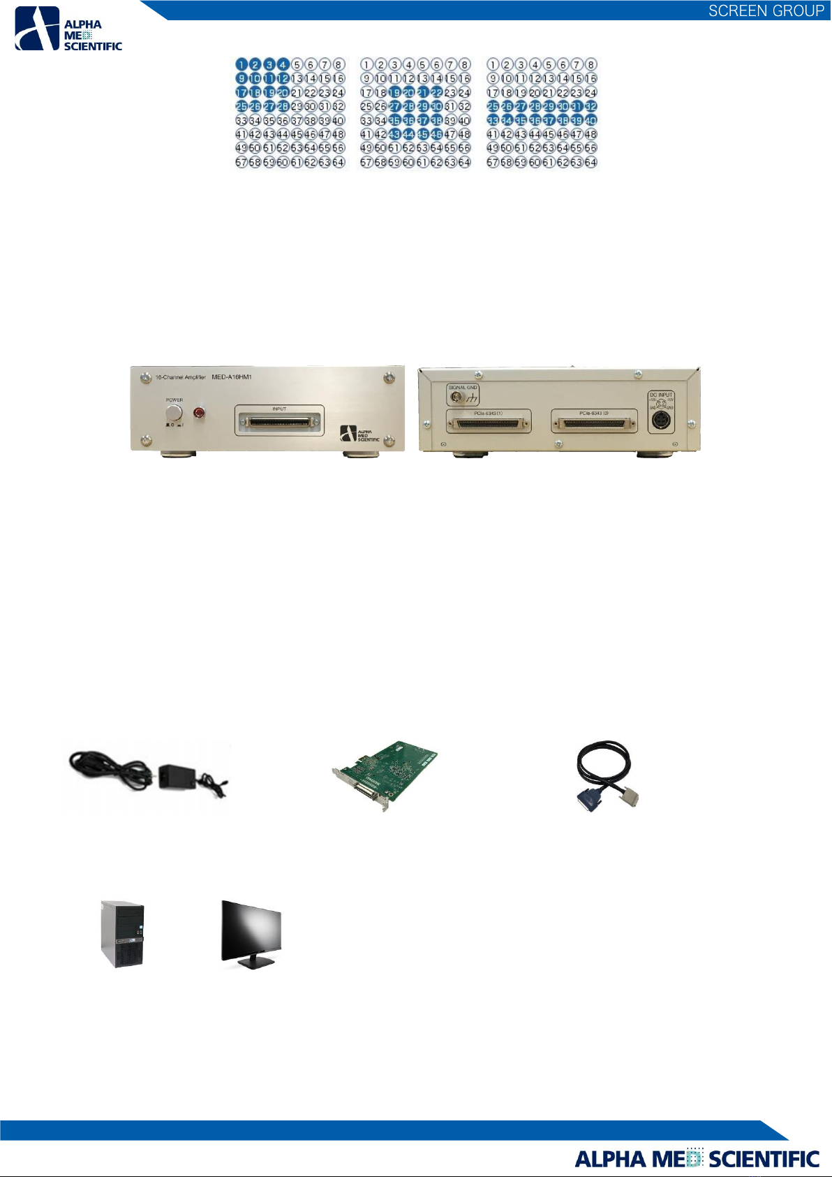
2.1.1. MED64-Entry Amplifier ……………….. 2
2.1.2. Accessories of the MED64-Entry Amplifier ……………….. 2
3. Setup of the MED64-Entry ……………….. 3
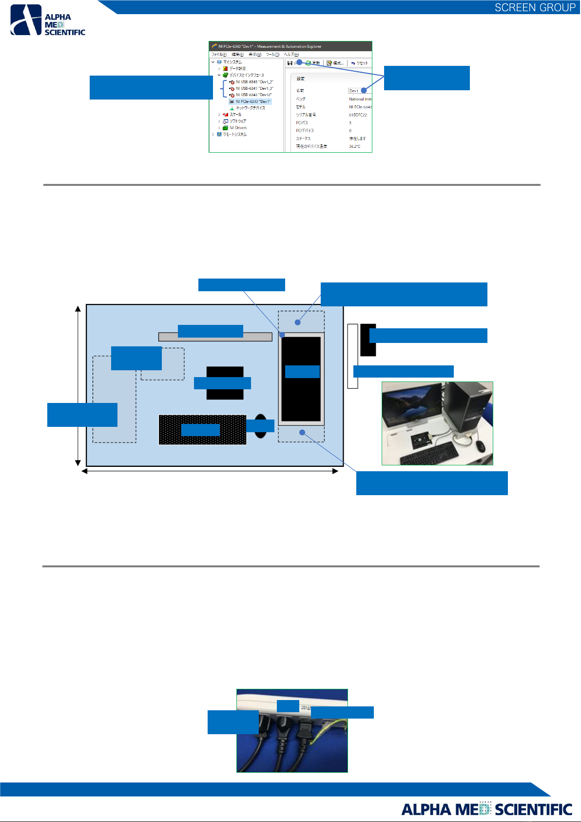
3.1. Connection of the data acquisition device to the PC ……………….. 3
3.2. Considerations for the position of devices ……………….. 4
3.3. Power source ……………….. 4
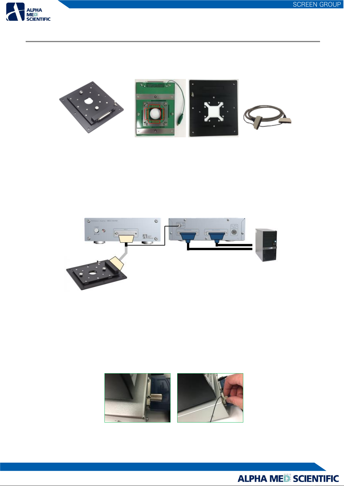
3.4. Connection to the MED64-Entry Amplifier ……………….. 5
3.4.1. Part names and functions of the MED Connector ……………….. 5
3.4.2. Connections of the MED Connector and the data acquisition device ……………….. 5
3.4.3. Positioning of the terminal of the MED Connector ……………….. 6
3.4.4. Electric shield with aluminum foil ……………….. 7
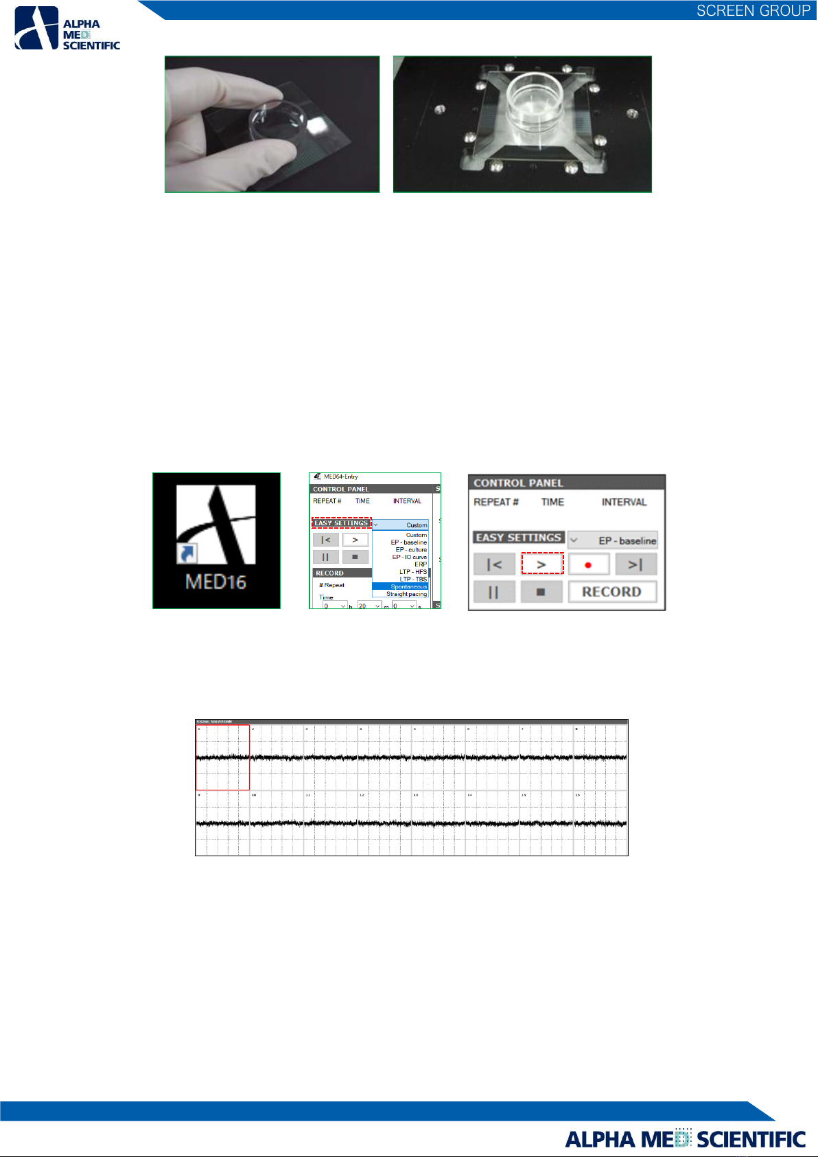
3.4.5. Preparation for the noise check -attaching the MED Probe ……………….. 7
3.4.6. Noise check ……………….. 8
3.4.7. Maintenance of the MED Connector ……………….. 8
4. Data acquisition by the control software “MED16” ……………….. 9
4.1. Setting the data acquisition schedule - RECORD subpanel ……………….. 10
4.2. Creating the stimulation pattern - STIMULATION subpanel and STIMULATION PATTERN tabs ……………….. 11
4.3. Set data file output - FILE OUTPUT subpanel ……………….. 13
4.4. SIGNAL WAVEFORM panel ……………….. 14
4.5. BASELINE STABILITY panel ……………….. 14
4.6. Replaying data file output - function of REPLAY mode ……………….. 16
5. Abnormal noise ……………….. 17
5.1. Noise check point ……………….. 17
5.2. Noise relation to installation ……………….. 17
5.3. Noise relating to perfusion ……………….. 19
5.4. Identification of cause when a malfunction of the device is suspected ……………….. 20
6. Appendix ……………….. 21
6.1. Specification ……………….. 21
6.1.1. MED64-Entry Amplifier [MED-A16HM1] ……………….. 21
6.1.3. MED Connector [MED-C03] and MED Thermo Connector [MED-CP04] ……………….. 22
6.1.6 Data Acquisition PC System ……………….. 22
6.2. Explanation of the technology ……………….. 23
6.2.1. Signal acquisition by the MED64 System ……………….. 23
6.2.2. Electric stimulation by the MED64 System - Applying current to the micro electrode array ……………….. 24
6.2.3. Stimulus artifact and biphasic stimulation ……………….. 24
6.2.4. Stimulus current value and electrolysis ……………….. 25
6.2.5. About the stimulus interval ……………….. 26

1
1. Introduction
◆ The MED64 system is a micro electrode array (MEA) system commercialized for the first time in the world in 1997. Since then,
the MEA system has been widely used in the United States and the EU for basic research in the fields of the central nervous
system and the cardiovascular system. Nowadays, its application to screening for drug discovery is rapidly spreading, thanks to
its highly evaluated excellent operability and efficiency.
◆ The system use a MEA with 64 planar electrodes arrayed in a pattern (MED probe) on a glass substrate. Users can acquire
extracellular potential simply by placing a tissue slice or by culturing cells on these electrodes. Current stimulation can be
applied through any electrode selected by software. Unlike a glass capillary electrode, the MED64 system requires no
troublesome operations to measure spontaneous activity or evoked response and no special training for electrophysiological
experiment is necessary. The system allows for accurate and easy measurements even by unexperienced researchers.
◆ The electrodes are made of platinum black or carbon nanotube with impedance 7 to 10 kΩ, the lowest impedance among
similar products on the market. The system is substantially free from external noise, thanks to its low impedance electrodes. It
needs no special environment/facility for electrophysiological experiment, such as a shield box, and it can be placed on a
laboratory desk for stable, daily measurement with no need for noise elimination.
◆ The MED64-Entry detects and amplifies extracellular potential using 16 out of 64 MEAs of the MED probe. The control software
“MED16” is specifically designed for data acquisition and after an experiment, the data obtained can be analyzed in various ways
by using the MED64 Offline toolkit.
2. Configuration of the MED64-Entry
The MED64-Entry Amplifier has a 68-pin SCSI cable terminal that can be connected to a MED Connector (MED-C03) or MED Thermo
Connector (MED-CP04). The amplifier has a channel selector circuit inside and acquires signals from 16 out of 64 electrodes of the
MED Probe in accordance with 1 of 3 patterns shown below (the pattern is defined at shipping).
MED64-Entry Amplifier
Data acquisition PC
Control software
“MED16”
MED Probe
MED Thermo
Connector
Headstage for MEA
Data acquisition
device (PCIe type)
MED Probe
MED Connector
OR
Multifunction
cable
68-pin SCSI cable

2
Type A Type B Type C
The extracellular potential detected at the recording electrodes of the MED probe is amplified 100 times by the MED64-Entry
amplifier and converted from an analog to a digital signal by a data acquisition device (National Instruments Corporation) with a
built-in PC. The signal acquisition and the application of the stimulation current is controlled by dedicated control software.
2.1. Part names and functions
2.1.1. MED64-Entry Amplifier
【Front】 【Back】
➊POWER ….. To switch ON/OFF of the power.
➋INPUT ….. An analog input terminal to input signals from the MED connector. It is connected to a connector terminal via the 68-
pin SCSI cable.
➌SIGNAL GND ….. A ground terminal to connect a lead for grounding.
➍PCIe-6343 ….. Output terminals to the data acquisition device (PCIe-6343, National Instruments Corporation). They are
connected to a VDHCI terminals of the data acquisition device on the back of the data acquisition PC via
multifunction cables (192061C-02, National Instruments Corporation). (0) is the output terminal for ch 1-8 (top
VDHCI terminal) and (1) is the output terminal for ch 9-16 (bottom VDHCI terminal).
➎DC INPUT ….. To connect to a power adaptor cord.
2.1.2. Accessories of the MED64-Entry Amplifier
➊ Power adaptor ➋ Data acquisition device (in the Desktop PC) ❸ Multifunction cable (1 m) x 2
2.1.3. Data Acquisition PC System
➊Desktop PC ➋Display monitor
❶
❷
➌
❹
❺
❹

3
3. Setup of the MED64-Entry
Thanks to the excellent electrode impedance (impedance of 50 µm electrode is 10 kΩ in frequency range 1 kHz) of the MED Probe,
which is the sensor of the MED64-Entry, the MED64-Entry offers several technological advantages:
1) Less influence by external noise (hum noise, etc.)
2) Very low Johnson noise (baseline noise) at about several µV
3) The MED Probe/Connector can be installed at a place physically distant from the amplifier (e.g., inside of an incubator with
100% humidity) via a 2 m connection cable, without being affected by noise or attenuation of the signal acquired.
A faraday cage or vibration isolation table that is typically necessary for an electrophysiological experiment is not necessary for the
MED64-Entry, but the MED64-Entry should be set up on a stable table without vibrations, such as a laboratory desk. A desk of about
100 cm width and 75 cm depth is necessary. For the user’s convenience, a larger desk is preferable. The power adaptor connected to
the amplifier, etc., serves as a magnetic field-derived noise source. When the MED64-Entry is set up on a desk against a wall, make
space for the cord between the wall and the desk and place the adaptor on the floor in order to place the power adaptor at a
distance from the amplifier and other components (the desk must not be fixed to the wall). Alternatively, a space is necessary to
ensure sufficient distance between the MED64-Entry and the power adaptor.
3.1. Connection of the data acquisition device to the PC
Note: For the MED64-Entry marketed in Japan, the process explained in this section is completed before shipment.
Open the housing of the PC, remove the extension slot cover on the back, and attach and fix with a screw the PCIe-6343 to the PCI
Express x1 slot on the mother board.
Run the NI-DAQ mx installer (ver. 16.0 or later) on the accessory DVD of PCIe-6343 to install NI MAX to the PC and connect the
MED64-Entry amplifier to the PC using a multifunction cable.
Launch NI MAX to confirm the configuration of the device. If a data acquisition device other than the PCIe-6343 was previously
connected to the PC, assign the name “Dev1” only to PCIe-6343 and assign other names to any other devices (on the control
software, “Dev1” is used as the identification code of PCIe-6343).
Expansion slot
cover
PCI Express x1
slot

4
3.2. Considerations for the position of devices
In order to ensure sufficient space for an experiment, place the PC on the MED64-Entry amplifier (not essential). Pay attention so
as not to damage the housing of the MED64-Entry Amplifier with the legs of the PC. Place the display monitor next to the PC and
the MED Connector in front of the monitor. Do not place the power adaptor or other electronic devices close to the connection
terminal on the back of the amplifier.
Above is an image of the ideal positions of components. The user can perform an experiment smoothly when there
is a sufficient space next to or at the back of the laboratory desk with a power strip on the floor. If no perfusion
system is used, about 100 cm width is sufficient, otherwise a larger space is necessary.
3.3. Power source
Three power sources are necessary for the MED64-Entry Amplifier and the Data Acquisition PC System (the desktop PC and the
display monitor), and one additional power source is necessary to use the MED Thermo connector when it is used. Connect all the
cords to one power strip connected to a wall outlet with the ground terminal (do not use an outlet on the desktop rack because it
is often not grounded properly). Do not connect devices that are not necessary for the MED64-Entry to the power strip or to the
wall outlet to which the MED64-Entry and other components are connected. Place the power cable and the power adaptor at a
distance from the amplifier, the MED Connector and the 68-pin SCSI cable.
Display monitor
PC
MED64-Entry
Amplifier
Space for cables on the back of the amplifier
About 20 cm depth is necessary.
MED Connector
Mouse
Keyboard
PC
Display monitor
Power strip (on the floor)
Power adaptor (on the floor)
75 cm
120 cm
アンプ後面
Data acquisition device other
than PCIe-6343 (not connected).
Save after assignment
of the name.
Space for cables in front of the amplifier
About 15 cm depth is necessary.
Pump (when
perfusing)
Water bath
(when perfusing)
MED64-Entry Amplifier

5
3.4. Connection to the MED64-Entry Amplifier
3.4.1. Part names and functions of the MED Connector
【Top unit】 【Base plate】 【Accessory】
➊Output terminal ….. To connect to INPUT of the MED64-Entry Amplifier via the accessory, the 68-pin SCSI cable.
❷Fixation screw ….. To fix the fitted top unit and the base plate with a MED Probe attached.
❸Contact pin ….. To contact with the MED Probe terminal to read signals.
❹Ground wire with an bagworm clip ….. To connect to a platinum wire with a perfusion cap when a perfusion system is used.
❺68-pin SCSI cable (2 m) ….. A conductive cloth tape and ground wire are wounded on the cable.
3.4.2. Connections of the MED Connector and the data acquisition device
➊Connect the output terminal of the MED Connector and the INPUT terminal of the MED64-Entry Amplifier, using the 68-pin
SCSI cable.
➋Connect the lead of the 68-pin SCSI cable to the SIGNAL GND terminal of the MED64-Entry Amplifier.
Note1: The 68-pin SCSI cable is wound with a conductive cloth tape and an uncoated lead is wound on it. If the other side of the
lead is free, the conductive cloth tape may serve as an antenna that collects electric noise and may cause noise. Make sure
that the other side of the lead is connected to the SIGNAL GND terminal of the MED64-Entry Amplifier (to use the
conductive cloth tape as an electric shield).
Note2: In order to prevent noise, use the SIGNAL GND terminal of the MED64-Entry Amplifier for single-point grounding when
the peripheral devices are grounded.
Loosen the screw of the SIGNAL GND terminal, insert the ground wire into the hole (left panel), and fix with a screw (right panel).
➌Connect the PCIe-6463 (1) terminal of the MED64-Entry Amplifier to the PCIe terminal (bottom) on the back of the PC, using
the function cable.
❶
❹
❶
❷
❸
❹
❺
❺
❷
❷
❸

6
➍Connect the PCIe-6463 (0) terminal of the MED64-Entry Amplifier to the PCIe terminal (top) on the back of the PC, using the
function cable.
➎Connect the power adaptor to the MED64-Entry Amplifier.
3.4.3. Positioning of the terminal of the MED Connector
Place the MED Connector with its output terminal and the 68 pin SCSI cable on the right side. In this position, the left top of the
MED Probe is assigned to ch 1 and the right bottom is assigned to ch 64. The orientation of the MED Probe is important because
the electrode number of the MED Probe is defined by the contact pins of the MED Connector.
Correspondence between the contact pin of the MED Connector and the electrode number: correspondence from the contact surface side with
the output terminal on the right (left panel) and correspondence with the MED probe terminal (right panel). R indicates the reference electrode.
Correspondence between the MED Connector output terminal and the electrode number. R indicates the reference electrode.
ch 1
ch 64
ch 56
ch 8
R1
R2
R3
R4
ch 1
ch 64
ch 56
ch 8
(0)
(1)
(0)
(1)

7
3.4.4. Electric shield with aluminum foil
If a noise check reveals that external electric noise is affecting the MED Connector, the noise may be avoided by placing a sheet of
aluminum foil under the MED Connector and using a lead to connect the aluminum foil sheet and the SIGNAL GND terminal of
the MED64-Entry Amplifier for grounding.
A sheet of aluminum foil serves as an electric shield by grounding. Magnetic field-derived noise cannot be prevented by an electric shield.
Note: Although the MED Connector is made from aluminum, its surface is coated and insulated from the aluminum foil. Make
sure that the aluminum foil is grounded to the SIGNAL GND terminal of the MED64-Entry Amplifier when a sheet of
aluminum foil is placed under the MED Connector, even if the baseline noise level is within an acceptable range. Without
grounding, the aluminum foil serves as an antenna to collect electric noise and may generate unexpected noise.
MED64-Entry after setup. In this example, the PC is placed on the right side.
3.4.5. Preparation for the noise check – attaching the MED Probe
Loosen the fixation screw of the MED Connector to remove the top unit.
On the base plate, place the MED Probe filled with saline, such as aCSF or PBS holding the ring chamber of the MED probe or the
end of the glass substrate. Pay attention so as not to touch the terminals. If any waterdrop, medium or smudge is on the terminal,
wipe the terminal with a Kim wipe before setting the MED Probe. Subsequently, place the top unit on the MED Probe and fix with
a fixation screw.
Fixation
screw
Top unit
Base plate
Fixation
screw

8
Note1: Loosen/tighten both screws little by little at the same time. When the screws are sufficiently loosened/tightened, they can
be completely loosened/tightened one by one. If only one screw is completely tightened/loosened without
tightening/loosening the other screw, the second screw cannot be inserted perpendicular to the hole.
Note2: Do not touch the contact pin of the MED Connector with bare hands. If sebum of the hand attaches to the pin, contact
impedance between the contact pin and the terminal of the MED Probe will increase and may cause noise. Pay attention
so as not to spill liquid (saline, medium etc.) on the MED Probe after it is set. Prevent liquids from coming into contact
with the contact pin.
3.4.6. Noise check
Double-click the MED16 icon on the desktop to launch the control software “MED16”. Select Spontaneous from EASY SETTINGS
and click the replay button.
Data acquisition will start 5 seconds later and the baseline noise will be displayed. The ideal baseline noise level is about ±8 µV
peak-to-peak. When baseline noise shows a normal pattern, the setup ends. For the details of operating the MED16 refer to p. 9
“Data acquisition by the control software” Refer to the relevant application note for the preparation of specimens used for the
experiment.
Normal baseline noise.
3.4.7. Maintenance of the MED Connector
A printed circuit board onto which 68 contact pins contacting the terminal of the MED probe are soldered is fixed by screws to
the top unit of the MED Connector. Spring-loaded pins are used as contact pins and keeping the surface of the pins clean is
important for the maintenance of the MED Connector. If any abnormal noise is found at a particular electrode and noise persists
on that electrode even when the orientation of the MED Probe is changed, the noise may be caused by deformation (crushing)
due to the wear of the contact pins associated with everyday use or dust or sebum on the contact pins. In the latter case, the
noise may be reduced by wiping the contact pin by pushing the eyeglass cleaner cloth on the pin. Do not use ethanol because
the contact pin is filled with lubricant for the spring. The printed circuit board needs to be replaced (paid repair) in the case of
malfunction due to wear of the contact pin associated with everyday use or malfunction due to salt (perfusion solution or media)
attached on the pin.

9
4. Data acquisition by the control software “MED16”
Turn on the power of the amplifier, the PC and the display monitor. Launch the control software by double clicking the MED16 icon
on the desktop. The software has two modes; RECORD mode to acquire data and REPLAY mode to replay the data file output
already. The MED16 starts in the mode that was used in the last session. At the first use, it starts in RECORD mode.
Main window of data acquisition in RECORD mode
The Main window of the RECORD mode has 4 panels.
CONTROL PANEL ….. To set conditions for data acquisition. It has the sub-panels of RECORD, STIMULATION and FILE OUTPUT.
STIMULATION PATTERN ….. To display the stimulation pattern set in the CONTROL PANEL.
SIGNAL WAVEFORM ….. To display the signal waveforms of all 16 electrodes during data acquisition.
BASELINE STABILITY ….. To display an enlarged view of the signal waveform of 1 electrode selected on the SIGNAL WAVEFORM
panel. From the signal waveform, it calculates a measure that indicates the stability of the activity or
response of the biological specimen, and it displays it as a time chart. BASELINE STABILITY has three
modes; Spike, EP and ISI. In Spike mode, the calculation is based on the frequency of spike detection; in EP
mode, the calculation is based on amplitude value of the evoked potential; and in ISI mode, the
calculation is based on the interval of the spike detection. None of the modes is intended for data analysis,
but the calculation in each mode provides information to help determine the timing of experimental
manipulation, such as the application of electric stimulation or the administration of a drug.
After setting the condition for data acquisition in the RECORD or STIMULATION (only for experiments using electric stimulation)
subpanel on the CONTROL PANEL, start the data acquisition by executing the software using the control button described below.
CONTROL
PANEL
SINGAL WAVEFORM
STIMULATION
PATTERN
BASELINE STABILITY
RECORD
STIMULATION
FILE EXPORT
When the elasticity of the pin
decreases, irreversible contact
failure occurs.

10
This software has 9 formats predefined for data acquisition assuming a standard experiment and EASY SETTINGS can call up one of
these formats (refer to p. 12 “Menus in EASY SETTINGS” for details). When the software starts, Custom is called up from these nine
pre-defined conditions.
Each panel has fields in the form of a text box or pull-down menu to define the condition. From the gray pull-down menu in the
figure below, users can only select one condition from the predefined values, while from the white pull-down menu, users can
directly enter any numerical value (the central panel in the figure below). The click button changes its color according to whether
on, off or invalid (the right panel in the figure below).
After defining the condition on the CONTROL PANEL, data acquisition is controlled by the control button on the upper part of the
CONTROL PANEL. The detailed conditions set on each panel are explained in the sections below.
Note1: Do not start other software during the data acquisition because it may place an unexpected load on OS and cause it to
freeze or to force a shutdown. Especially, you need to pay attention to software running background, such as anti-virus
software. Do not connect to the Internet, because it may place an unexpected load due to the communication and cause it
to freeze or to force a shutdown.
Note2: In this document, data acquisition with data file output is called “record.”
4.1. Setting the data acquisition schedule – RECORD subpanel
The data acquisition schedule consists of 1 or more data acquisition sessions (called “repeat” in this software) set arbitrarily by the
user on the RECORD subpanel. In the example shown below, a session (repeat) consisting of 0.1 s data acquisition and 19.9 s
waiting time is repeated 1,000 times. The minimum increment for Time (data acquisition) is 0.1 s and for Interval (repeat) is 1 s. The
value of Interval must be at least 0.1 s higher than the value of Time.
On
Off
Invalid (cannot be clicked)
Control button
|< Replay one previous repeat. This button is not used
for a record.
> Acquire data without outputting the data file.
● Acquire data while outputting the data file (record).
>| Replay one repeat forward. This button is not used
for a record.
|| Pause data acquisition between repeats.
■ Stop data acquisition.
Displays current mode.
Click to switch mode.
Displays time elapsed
during data acquisition.
Calls up predefined condition
for data acquisition.
Value can be
directly entered
Only selections from
predefined values are
available

11
The maximum input voltage is entered to Max input. When a signal exceeding the set value is input during recording, the set value
is acquired as the saturated value. Digitizer resolution is 16 bit in the MED64-Entry, which follows that the resolution of the voltage
value is a value obtained by dividing Max input by 216. Set an appropriate value according to the magnitude of extracellular
potential obtained from the biological specimen. High pass filter or Lowpass filter is not applied to the data file output. Instead,
they are applied to the displayed raw waveform in OSCILLOSCOPE or RAW WAVEFORM - SELECTED ELECTRODE during data
acquisition.
4.2. Creating the stimulation pattern – STIMULATION subpanel and STIMULATION PATTERN tabs
The STIMULATION subpanel has 3 tab windows; Step 1, Step 2 and Manual. When either Step 1 or 2 is enabled and the stimulation
pattern is set in that tab, the pattern is applied to all repeats. If both Step 1 and 2 are enabled and stimulation pattern is set, the
pattern is applied alternatively for each repeat. For repeat 1, stimulation pattern of Step 1 is applied; for repeat 2, stimulation
pattern of Step 2 is applied; for repeat 3, stimulation pattern of Step 1 is applied, and so on (see the right panel of the figure
below). Because the MED64-Entry Amplifier has 2 terminals (S1 and S2) for stimulation output, the stimulation pattern is applied to
up to 2 electrodes in one Step.
Schematic drawing of data acquisition and stimulation pattern. In this example, a stimulus is applied to 1 electrode in Step 1 and a
different stimulus is applied to the other 2 electrodes in Step 2.
Note: The length of the stimulation pattern must not exceed the length of Time.
The Manual tab has a Start Stim button enabled only during the pause between repeats. When the Start Stim button is clicked, the
stimulation set in the Manual tab can be applied manually at any time. When the stimulation is applied during the recording of
data, the data file for that interval is output as a separate file.
The minimum unit composing a stimulation pattern is a biphasic pulse or a monophasic pulse. A stimulation pattern is composed
by coupling 1 or more stimulation pulse set at the Pulse config.
Repeat # 1
Repeat # 2
Repeat # 3
Time
(acquisition)
Interval
Interval
Interval
・・・
Repeat # 1
Repeat # 2
Repeat # 3
Repeat # 4
Time
Time
Time
Time
Interval
Interval
Interval
Interval
S1
S2
Step 1
Step 2
Step 1
Step 2
Step 2
Step 2
not set
not set
Check to enable
“#” is added before and after the
tab name for the invalid step.
Tab menu
Time
(acquisition)
Time
(acquisition)

12
In the Pulse type, Biphasic (biphasic pulse) or Const (monophasic pulse) is selected. Usually, select Biphasic. In Duration, the pulse
width is specified in 0.1 s increments. When Biphasic is selected, 50% of the specified value is applied to each phase. In Intensity, a
positive or negative integer is specified. When Biphasic is selected, the designated value is assigned to the first phase and the
value with an inverted sign is assigned to the second phase. In Pre and Post, the waiting time before and after a pulse is specified
in 0.1 s increments. For the reason why a biphasic pulse is selected, refer to p. 24 “6.2.3 Stimulus artifact and biphasic stimulation.”
Note: In order to return the output current of the stimulation pulse to the 0 level, be sure to set the Post value for the last pulse of
the stimulation pattern.
The Pulse config represents 1 pulse range of a stimulation pattern. A stimulation pattern is composed by clicking the buttons
shown below to add, delete or repeat 1 pulse range to the whole stimulation pattern.
Menus in EASY SETTINGS
Custom ….. When the software is closed while Custom is selected, all the defined data acquisition condition can be stored and
called up at the subsequent launching of the software. This menu is provided for the user’s convenience and users can
repeatedly use the specific data acquisition condition defined by themselves without having to define it again.
Note: In menus other than Custom, the condition defined by the user cannot be stored. Default values are called up
every time the software is launched.
EP - baseline ….. This menu is provided for recording the evoked response (the evoked potentials) in a brain slice. A session
consisting of 0.1 s data acquisition and 19.9 s waiting time is repeated 1,000 times. Max input is set at 10,000 uV
and the data in bandwidths 1 to 10,000 Hz are shown. For example, for an acute hippocampus slice, it is in good
condition if amplitude ≥-300 uV is obtained by a default stimulation pulse (0.2 ms width, -10 uA) (an estimated
value).
Pulse type
Electrode to which the stimulation pattern is applied
(it cannot be set for an individual pulse)
Pulse #
#1
#2
#3
#4
Pre
Post
Duration
Pre and post pulse
time
Pulse duration
Stimulus intensity
The pulse designated by Pulse # or selected
by a direct click on the STIMULATION
PATTERN panel is highlighted in red.
Pulse selected is deleted.
Specified number of a pulse
set in Pulse config is added
after the pulse selected.
Stimulation intensity specified in
Increase intensity is applied to all
units.
The stimulation intensity specified in
Increase intensity is accumulatively applied
for each repeat to all units.
This button is always on or off.
The stimulation pattern defined is
repeated continuously in a repeat.
This button is always on or off.
Intensity
Const
Biphasic
1st phase
2nd phase

13
EP - culture ….. This menu is provided for recording the evoked response (the spike) in a dissociated neural culture (cultured neural
network). A session consisting of 0.1 s data acquisition and 4.9 s waiting time is repeated 100 times. Max input is
set at 10,000 uV. A low frequency component may be generated at baseline by LFP (local field potential) caused by
spontaneous activity, and filtering is applied to bandwidths 100 to 10,000 Hz to allow for the easy observation of a
spike. Whether a spike is evoked or not by a default stimulation pulse (0.1 ms width, -20 uA) at any electrode in a
constant delay time from stimulation artifact is observed while switching the stimulation electrode. When no
evoked spike is observed at any stimulation electrode, repeat the same procedure with the stimulation intensity
increased (e.g., -30 uA).
EP - IO curve ….. In this menu, the input-output relationship (the input-output curve of the evoked potentials relative to the
stimulation intensity) is recorded in a brain slice. The data acquisition condition is almost the same as the EP-
baseline, but the stimulation intensity is increased by 1 uA for every 1 repeat because by rep # it is enabled. The
number of repeats is set to 90 because the max stimulation intensity is 100 uA. The data acquisition is stopped
manually when a saturation response is obtained.
ERP ….. This menu is provided for recording the effective refractory period by premature stimulation in a dissociated
cardiomyocytes. Electric stimulation with width 0.6 ms, intensity -10 uA and basic cycle length (interval between pulse)
1,000 ms is applied 10 times, followed by the 11th electric stimulation with a shorter cycle length of 900 ms.
LTP - HFS ….. This menu is provided for LTP induction by tetanus stimulation. The data acquisition condition is almost the same as
the EP - baseline, but tetanus stimulation with 10 ms interval (100 Hz) for 1 s (100 stimulation) is set in the Manual
tab. The default stimulation intensity is -20 uA. To change the value to a value defined based on the result of the
input-output relationship, enter the difference between the default value and the new value in Increase intensity, and
click on the in all units button to increase/decrease the stimulation intensity for the stimulation patterns as a whole.
LTP - TBS ….. This menu is provided for LTP induction by θ burst stimulation. The data acquisition condition is almost the same as
the EP - baseline, but 4 pulse stimulation of 100 Hz is set at 200 ms (5 Hz) interval for 2 s (10 times) in the Manual
tab. The default stimulation intensity is -20 uA. To change the value to a value defined based on the result of the
input-output relationship, enter the difference between the default value and the new value in Increase intensity, and
click on the in all units button to increase/decrease the stimulation intensity for the stimulation patterns as a whole.
Spontaneous ….. Data in the bandwidths 1 to 10,000 Hz is acquired with Max input 10,000 uV. Data for continuous 20 m interval is
acquired with no stimulation.
Straight pacing ….. This menu is provided for recording the paced responses in a fixed cycle for a cardiac culture. Repeat all the
time is enabled and pacing is applied continuously at stimulation width 0.6 ms, stimulation intensity -10 uA, and
cycle length (interval between pulses) 1,000 ms. To change the cycle length, edit the value in Post.
Note: When any menu is called up from EASY SETTINGS and switched to Custom, the Custom takes over the acquisition condition
of that menu.
4.3. Set data file output – FILE OUTPUT subpanel
When data acquisition is executed by the record button, a data file is generated after the data acquisition. The folder to output
and the file name are specified in the field shown in the figure below:
In RECORD mode, the output format of the data file cannot be specified and the file is output in a unique .endat format. The file
name is automatically assigned in the format “Year Month Date_####h##m##s(_added text).endat.”
Must be specified. If no folder is
specified before data acquisition, a
prompt window appears.
Optional item. Text to be added to
the file name is entered.
The format of the data file to be
output is specified. The format
cannot be specified for recording
(it can be specified for replay only).

14
4.4. SIGNAL WAVEFORM panel
The signal waveform (raw data) is depicted for all 16 electrodes. Select one electrode (in the red frame) by left clicking on the chart
of the electrode to show the waveform for that electrode on the BASELINE STABILITY panel.
Right clicking on the panel calls up the menu to switch the display of the electrode array pattern or the scope of the display of the
axis common to the electrode charts.
Each electrode chart is divided by auxiliary lines into 5 divisions on the X axis and 4 divisions on the Y axis. The values specified on
the right-click menu X-axis and Y axis indicate the display time (ms/div) and the voltage (uV/div) per division. The voltage specified
is a positive/negative value with 0 uV as the center. By selecting On in Autoscale, the Y axis is automatically adjusted in 2.5 s
increments for each electrode, based on the maximum voltage value. Copy Image copies the panel image onto the clipboard.
In Preferences, Line Color customizes the color of data points, Background Color customizes the background color of the chart and
Grid Color customizes the color of the auxiliary lines. By selecting Default, the changes are returned to the default values.
4.5. BASELINE STABILITY panel
The stability of the activity of the biological specimen is shown on the monitor. There are 3 modes to select–EP, SPIKE and ISI– each
of which has a different measure as the indicator of activity. The upper panel shows an enlarged view of the signal waveform of the
electrode selected in the SIGNAL WAVEFORM panel, and the range to calculate the measure is specified by the cursor. The lower
panel shows a time chart of the measure calculated.
BASELINE STABILITY panel in EP mode
Mode switching button
To search minimum value between cursors
Signal waveform
Measure

15
In EP mode, two perpendicular cursors appear on the signal waveform chart. Use drag & drop to change the position on the X-axis
and calculate the minimum value of the raw data between the two perpendicular cursors to obtain the indicator of stability of
activity.
SPIKE mode (left) and ISI mode (right) of BASELINE STABILITY panel.
In SPIKE mode or ISI mode, one horizontal cursor (threshold) appears on the raw data chart. Use drag & drop to change the
position on the Y-axis, to count the frequency of the signal crossing with the threshold (SPIKE), or to calculate the interval between
crossings (ISI: inter-spike interval). The target of the measure is the cross point for rising when the threshold is on the positive side,
and the cross point for falling when the threshold is on the negative side.
The same as in the SIGNAL WAVEFORM panel, a menu to change the scope to display on an axis appears by right clicking on the
signal waveform chart. The value specified on the X-axis indicates the maximum value (s) on the X-axis. For the Y-axis, click the axis
label of the extreme value to change the scope of display by direct editing.
Other menus are the same as those available in the SIGNAL WAVEFORM panel.
The measure chart is similar to the signal waveform chart. Step Filter shows only the evoked response at either step as a time chart,
for data acquisition with Step 1 and 2 enabled. Copy Data stores the numerical data of the time chart on a clipboard. Moving the
mouse cursor over each plot of the chart shows the numerical information of that plot point.

16
4.6. Replaying data file output – function of replay mode
This software has a replay mode to check a recorded data file.
Main window of REPLAY mode.
As shown in the figure above, the screen looks almost same as that of RECORD mode, except for some differences in the
CONTROL PANEL. The data file to be replayed, the scope of replay and the number of electrodes are specified on the REPLAY
subpanel. To convert and output a data file in an endat format to a binary format or csv format, specify accordingly on the FILE
OUTPUT subpanel.
When the data file name appears in Filename field, replay the data file using the control button. To convert the data file format to
be output, execute the software using the record button.
The MED16 has limited functions for data analysis in order to reduce the load during operations. For data analysis, consider using
the MED64 Offline Toolkit or the separately sold MED64 Burstscope and MED64 Peakmap that are compatible with the endat
format. Refer to the product manuals of each product for further details.
Click to select a data file to replay. When the file name appears in the
Filename field, the file can be replayed using the control button.
Control button
|< Replay one previous repeat. This button is not used
for a record.
> Replay data without outputting the data file.
● Replay data while outputting the data file (record).
>| Replay one repeat forward. This button is not used
for a record.
|| Pause replaying data between repeats.
■ Stop replaying data.
Displays current mode.
Click to switch mode.
Displays time elapsed
during replaying data.
Calls up predefined speed for
replaying data.

17
5. Abnormal noise
5.1. Noise check point
- The amplitude of normal baseline noise has about ±8 µV peak-peak value in bandwidth between Low cut freq 1 Hz and High cut
freq 10,000 Hz for signal acquisition. Visually check whether the baseline noise is flat on the display with 20 ms/div on the
horizontal axis and a display 500 ms/div on the horizontal axis.
Normal baseline noise.
- For electrodes with noise, check whether noise occurs in a particular subset of electrodes or in all 16 electrodes and whether
there is any bias in the noise.
- For the shape of noise, set the horizontal axis at 20 ms/div and check whether the noise is a sinusoidal-like noise repeated 5 or 6
times or a high-frequency noise disproportionately observed in particular electrodes.
- There are two types of extrinsic noise; noise that can be shielded by an electric shield regardless of distance, and noise for which
an electric shield is not effective but can be reduced by moving the noise source to a distant position. The latter noise may be
caused by a magnetic field generated by a device connected to the power cable (power adaptor, perfusion pump, and water
bath, etc.). Move the responsible device to a position where the noise disappears or unplug the power cable of that device when
MED64-Entry is being used.
Note: To contact our help desk, select Copy Image by right clicking on SIGNAL WAVEFORM, paste the image of 16 electrode on an
image editor such as paint, store in jpg or tif format, and send it to the help desk as an e-mail attachment. Do not use bmp
format because it has a large file size. Prepare images with 20 ms/div and 500 ms/div horizontal axis and 25 µV/div vertical
axis, or a vertical axis automatically adjusted by Autoscale.
5.2. Noise relating to installation
- A fixation screw of the MED connector is loose.
An example of noise when a fixation screw is loose. Noise is likely to occur in all 16 electrodes.
20 ms
25 µV
25 µV
0.5 s

18
- Poor contact between the SCSI cable and the analog input terminal.
An example of noise when the contact of the SCSI cable is poor.
- The power adaptor or other electronic device (incubator, etc.) is placed close (about 30 to 100 cm) to the terminal of the MED64-
Entry Amplifier or the 68 pin SCSI cable.
Magnetic field noise caused by a nearby power adaptor. Beard-shaped characteristic noise. Interference (an effect of the
magnetic field) occurs in particular electrodes.
- A heater circuit or electromagnetic valve of the incubator operates and a magnetic field is generated inside the incubator.
An example of magnetic field noise caused by an incubator. Interference occurs in particular electrodes, the magnitude of
effect depends on the position in the incubator, and the noise disappears when the temperature is stabilized (an example
screen of the MED64-Basic to clearly show the disproportionate effect).
- A power cable of an electronic device not relating to the MED64 system is connected to the power strip, and the noise
disappears when the device is disconnected.