Applied Photophysics Chirascan CD User manual

2.1 Updated January 2006
ADDING
NEW
DIMENSIONS TO KINETICS
Chirascan
Quick Start
This guide provides an introduction to the use of the
Chirascan CD Spectrometer.
It covers the running of simple experiments
and the basic use of the software.
ADDING
NEW
DIMENSIONS TO KINETICS
Applied Photophysics Limited
203/205 Kingston Road
Leatherhead KT22 7PB
United Kingdom
Tel: [phone]
(USA) 1- 800 543 4130
Fax: [phone]
Email: [email protected]
URL: www.photophysics.com

2.2 Updated January 2006
Contents
2.0 Introduction................................................................................................................3
2.1 Purging.......................................................................................................................3
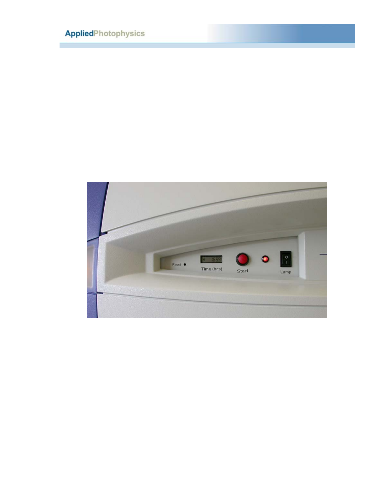
2.2 Power-up....................................................................................................................4
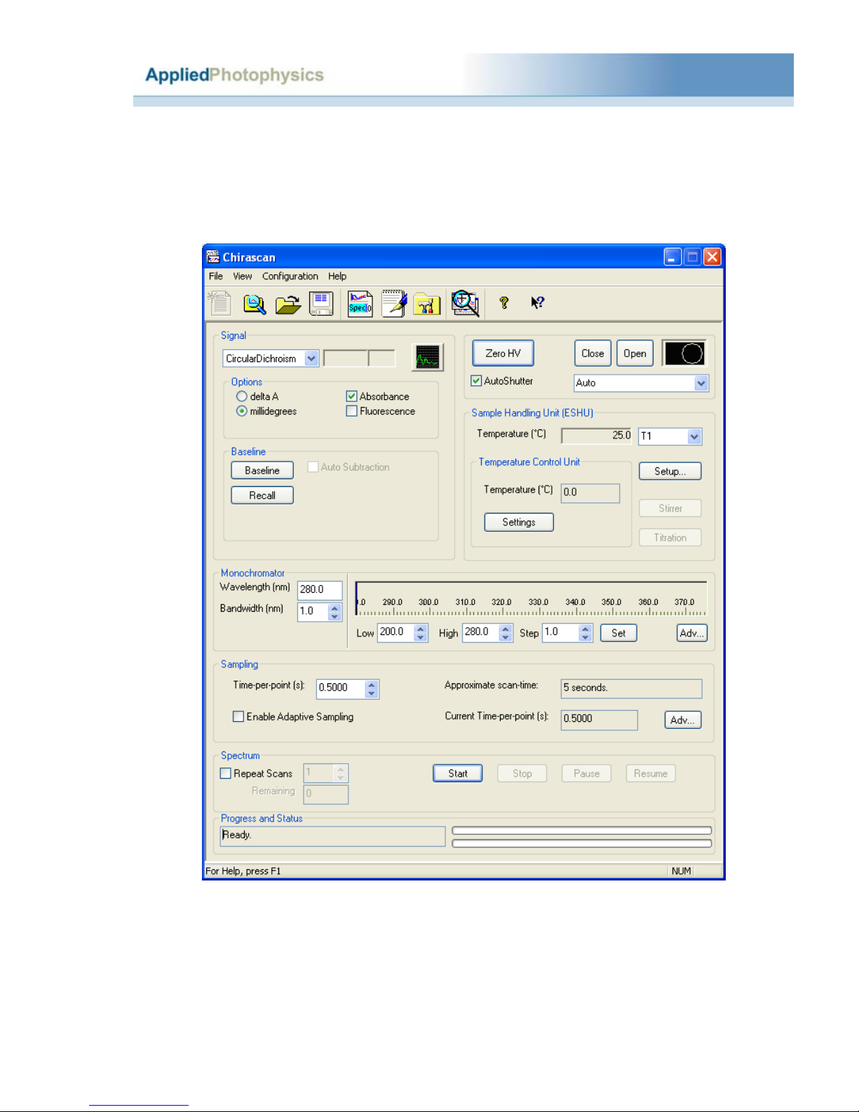
2.3 Launching the software..............................................................................................6
2.3.1 Measuring a CD baseline and spectrum..................................................................7
2.3.1.1 The CD baseline...................................................................................................7
2.3.1.2 The CD spectrum...............................................................................................10
2.4 Viewing and manipulating spectra and traces..........................................................11
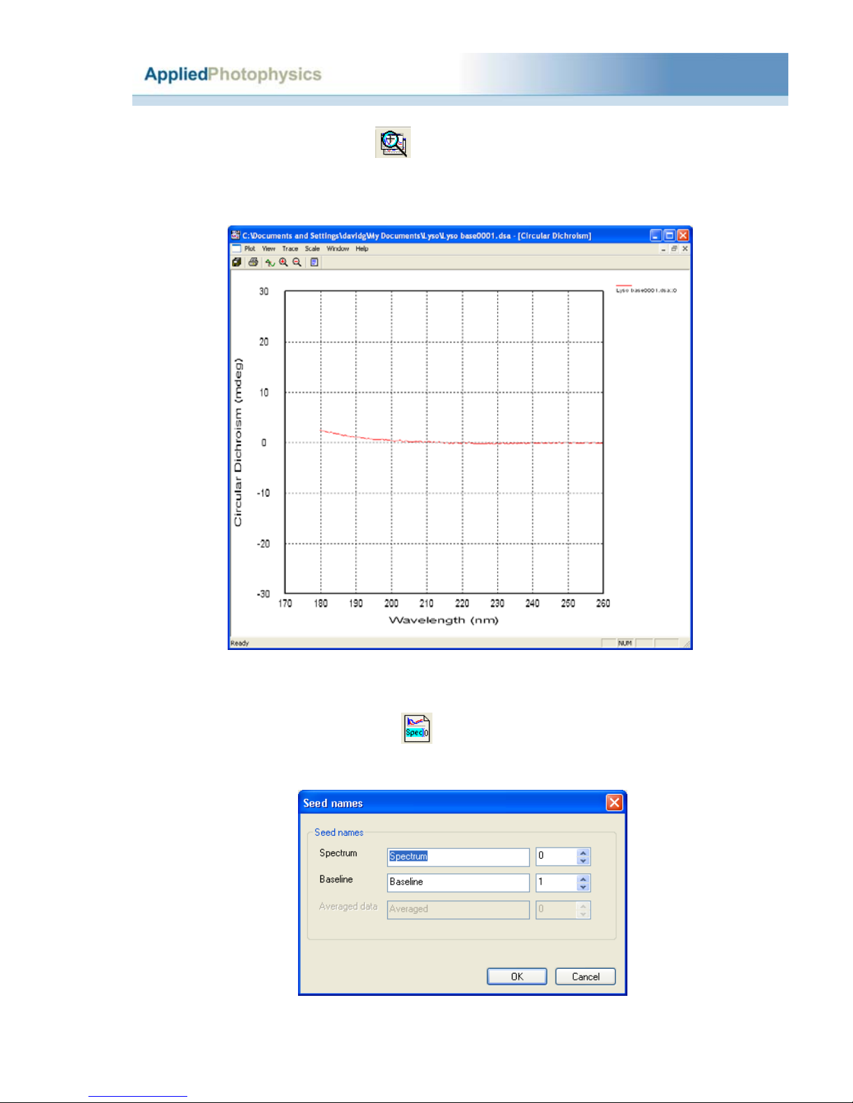
2.4.1 Viewing spectra ....................................................................................................12
2.4.2 Comparing spectra................................................................................................13
2.4.3 Manipulating spectra.............................................................................................14
2.4.4 Example of spectrum manipulation ......................................................................21
2.5 Saving data...............................................................................................................26
2.5.1 Converting data for use with third-party programs...............................................27
2.6 Printing.....................................................................................................................28
2.7 Operating notes and hints.........................................................................................28
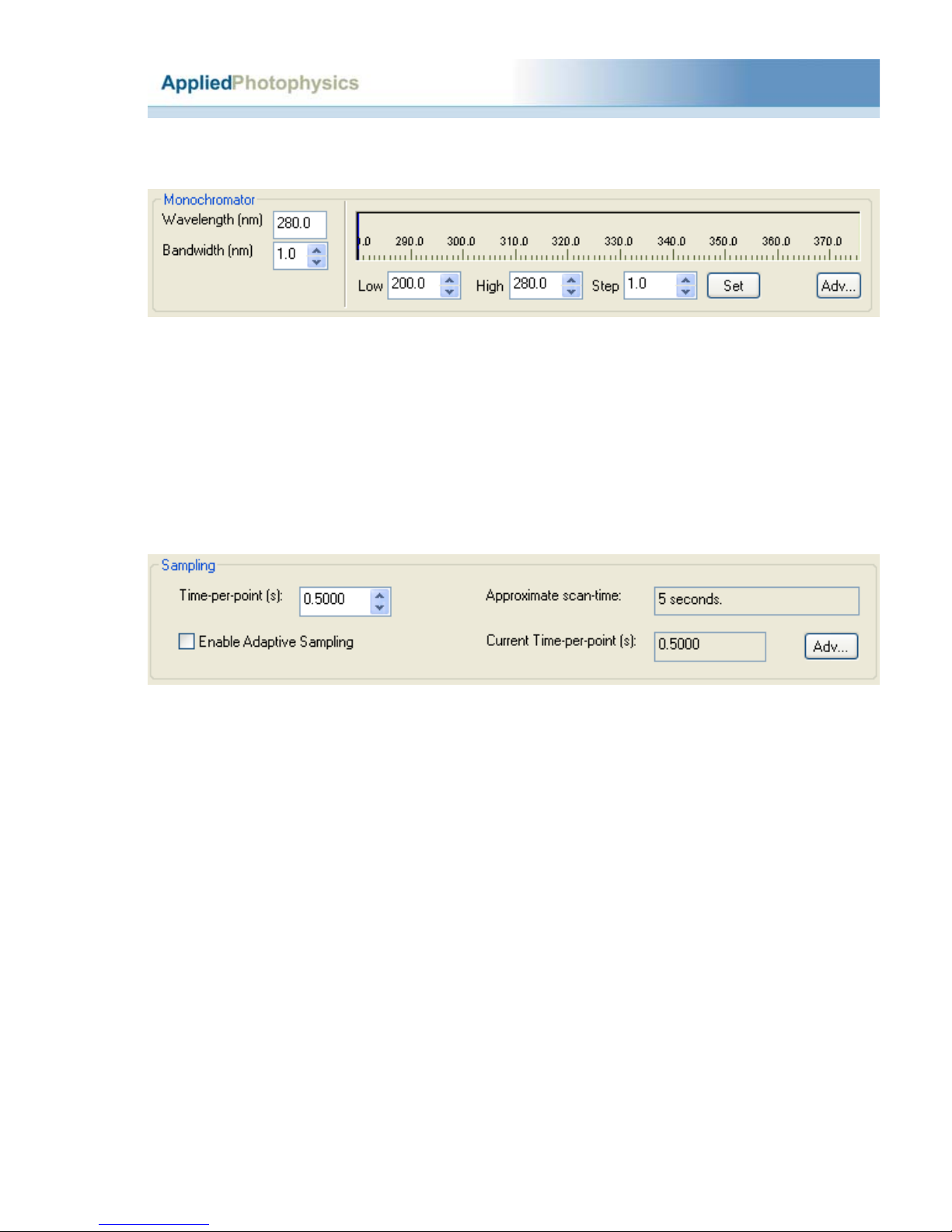
2.7.1 Selecting Step Size (SS)........................................................................................28
2.7.2 Selecting Spectral Bandwidth (SBW)...................................................................28
2.7.3 Selecting pathlength and concentration.................................................................29
2.7.4 Selecting time per point ........................................................................................29
2.7.5 Nitrogen purge flow-rate.......................................................................................30
2.7.6 Measuring protein spectra.....................................................................................30
2.8 Example spectra.......................................................................................................31
2.8.1 Alcohol dehydrogenase.........................................................................................32
2.8.2 Bovine serum albumin..........................................................................................33
2.8.3 Cytochrome C.......................................................................................................34
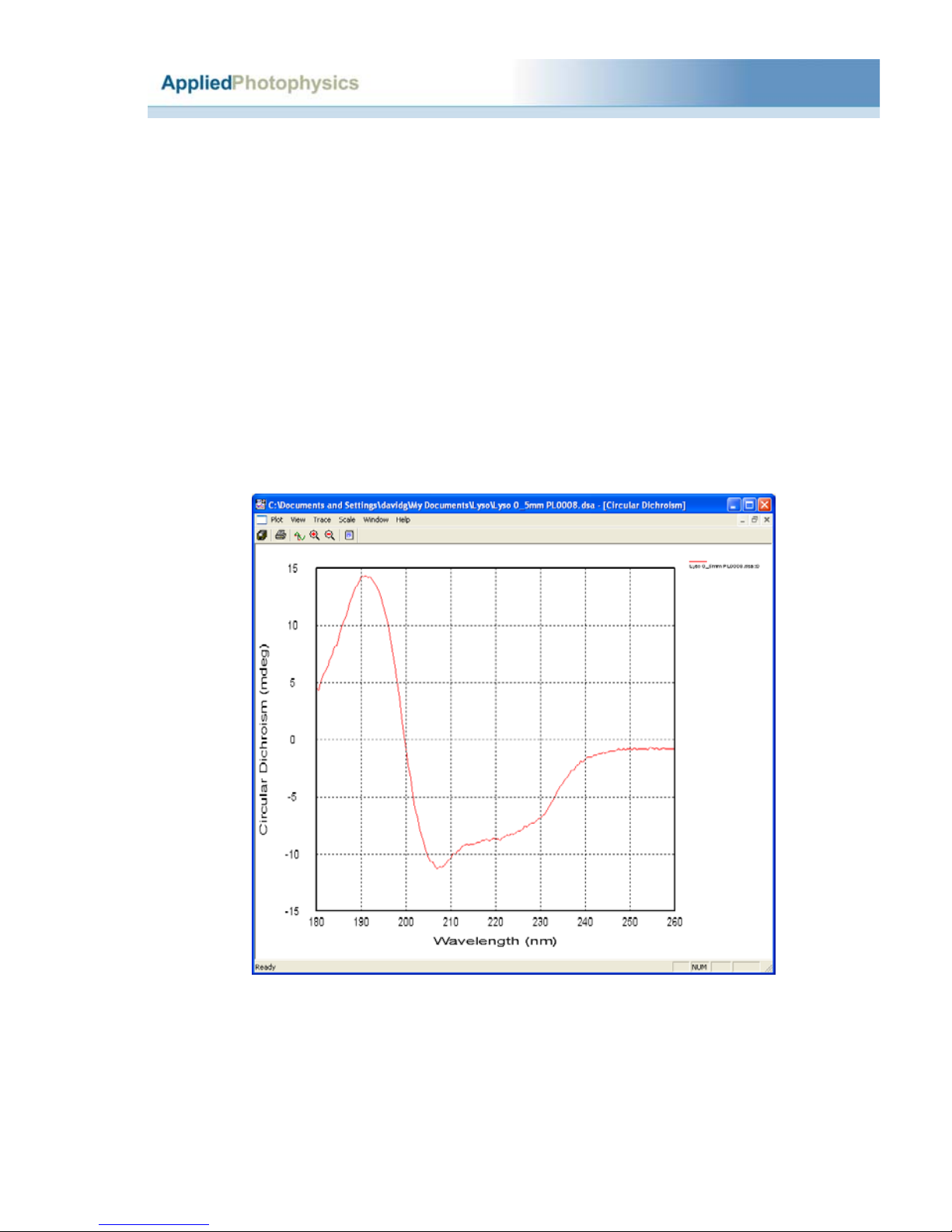
2.8.4 Lysozyme..............................................................................................................35
2.8.5 Vitamin B12..........................................................................................................36
2.8.6 Tris(ethylenediamine) cobalt chloride ..................................................................37
2.8.7 Camphor sulphonic acid........................................................................................38
2.8.8 (R)-3-methylcyclopentanone ................................................................................39
2.9 Troubleshooting.......................................................................................................40
2.10 Notes......................................................................................................................41

2.3 Updated January 2006
2.0 Introduction
APL recommends that new users read this guide to familiarise themselves with the basic
operation of the instrument. The operations covered are start up of hardware and
software, use of the Chirascan instrument control and data acquisition software to
collect CD spectra and baselines, use of the graphics software to carry out common
operations on the data and to save data appropriately and conversion of data formats for
export to third-party programs.
2.1 Purging
Removal of air from the light path by purging with nitrogen is essential, not
optional. Failure to purge the instrument will result in the formation of ozone,
which is damaging to health and can cause deterioration of the optical components
in the instrument.
The instrument is purged using clean nitrogen that is distributed to the instrument via a
manifold that contains three gas flow controllers (see picture below). The gas pressure
regulator of the master supply should be set in the range 2bar < P < 6bar, in accordance
with the manufacturer’s recommendation. At first start-up, set the gas flow as high as
the supply pressure allows, with most flow through the monochromator (middle) flow
controller, and let the purge to continue for at least 15 minutes prior to attempting to
ignite the lamp (see next section). After this initial, high-flow purge, the controllers can
be set at 1 Lmin-1 -1 -1
, 3 Lmin and 1 Lmin for the lamp housing, monochromator and
sample housing respectively.
Three rotameters (gas-flow controllers) control nitrogen flow to the lamp housing,
monochromator and sample housing respectively, from left to right.

2.4 Updated January 2006
The lamp housing and monochromator are hermetically sealed, which means that once
the initial purge is complete, you should not need to repeat the high flow-rate purge,
unless the hermetic seals are broken (during service or lamp replacement) or if the
instrument has been left idle for many days.
NB It is essential that the nitrogen used to purge the instrument be clean. APL strongly
recommends the use of a combined molecular sieve (X13) and activated charcoal gas
trap, which will remove from the nitrogen stream all common impurities, which can
otherwise deposit on the internal optical surfaces. The cleaner the nitrogen, the longer
your Chirascan will maintain its far-UV performance.
2.2 Power-up
Ensure that the instrument is connected to the electricity supply and that it has been
purged according to Paragraph 2.1. Put the two black rocker switches (System and
Lamp) on the front panels to the on (I) position. The instrument will automatically
check its zero positions (you may hear the monochromator motors moving). Ignite the
Xe arc lamp by pressing the red Start button on the lamp control panel no sooner than
20 seconds after the lamp power supply has been switched on – this is to allow
sufficient time for the capacitors to charge up. If ignition is successful, the translucent
panel on the source housing adjacent to the control panel will glow yellow; if you do
not see a yellow glow, press the red Start button again; repeat until ignition is achieved.
The lamp will require at least 15 minutes to stabilise following ignition. Finally, ensure
that the computer, its monitor and printer are all powered up.
The System panel

2.5 Updated January 2006
NB Once the lamp is struck, it is strongly recommended that it be left on for the
duration of the work planned for the day. Repeated powering up and powering down
will lead to instabilities (see previous paragraph) and will reduce the life of the lamp.
However, if it is necessary to restart the lamp after running, it must be allowed to cool
for about 15 minutes before re-ignition is attempted.
The light-emitting diodes (LED) on the System panel are labelled Status, Tx and Rx; Tx
and Rx will illuminate when commands are being transmitted or data is being received
respectively; the green Status LED should be constantly illuminated – if it is flashing, it
indicates that one or more of the electronics self-tests has failed. If this happens, try
restarting the electronics and if the problem persists, please contact APL technical
support.
The Lamp panel
The red LED on the Lamp panel indicates that power is present. The digital timer
records the number of hours that the lamp has been running; adjacent to the timer is a
recessed reset button: the timer must be reset when the lamp is changed.
On shut-down, it is recommended that only the lamp be extinguished by putting the
black rocker switch to the off (O) position. The electronics can be left switched on quite
safely. Once the lamp is extinguished, the nitrogen should be left on for a few minutes
while the lamp cools and because the lamp housing and monochromator are
hermetically sealed, there will be little or no loss of purging integrity overnight or even
over a weekend. Resuming normal nitrogen flow for 10 minutes after a weekend
shutdown is usually sufficient to re-establish a fully purged light path.

2.6 Updated January 2006
2.3 Launching the software
On starting the computer, among other icons on the desktop, you will see two associated
with the Chirascan. They are called Chirascan and Chirascan Viewer. Double-click on
the Chirascan icon to launch the Pro-Data interface.
The Pro-Data interface
The Pro-Data interface enables you to configure the instrument and to manage
experiments. It is divided into a number of sub-panels - Signal, Baseline, Sample
Handling Unit, Monochromator, Sampling, Spectrum and Progress - in which are
grouped the parameters relevant to the control or management of that sub-panel’s

2.7 Updated January 2006
function. In addition, there is an unlabelled panel for controlling shutter function and
detector high voltage.
2.3.1 Measuring a CD baseline and spectrum
NB When you put a sample into the sample chamber, it is inevitable that a small
quantity of air will be introduced to the low-volume light path within the purge tubes in
the sample chamber. It takes only a few seconds to re-establish an air-free environment
and you should not need to wait longer than that before starting your measurement.
2.3.1.1 The CD baseline
Every CD spectrometer has a CD baseline, caused by the interaction of circularly
polarized light (CPL) with the slight birefringence found in the PMT detector window
and to a lesser extent in the cuvette. To see the true CD spectrum of your sample, this
baseline must be measured and subtracted from the CD spectrum of the sample.
To measure the CD baseline, you must measure the CD spectrum of a blank. The blank
must be identical in every way to the sample that you want to measure, except that the
sample itself is absent. For example, if you intend to measure an aqueous solution of
lysozyme in a 0.2mm path-length rectangular cuvette, then the CD baseline is
determined using the same cuvette containing only water.
Signal panel in the Pro-Data interface
In the Signal panel, there is a drop-down menu that contains the main data collection
modes: choose Circular Dichroism. In Options, choose either delta A (delta absorbance)
or millidegrees, depending on the units in which you wish to express the CD
measurement. Select Absorbance if you wish to simultaneously measure the absorbance

spectrum of the sample. Note that Circular Dichroism, millidegrees and Absorbance are
selected by default.
Monochromator panel in the Pro-Data interface
Set the lower and upper wavelength limits of the scan range for your experiment in the
Monochromator panel of the Pro-Data interface – these will normally be the same for
both CD baseline and CD spectrum. For example, set Low to 180nm and High to 260nm
if you are measuring a typical protein. Set the wavelength step size in Step, typically
1nm or less, and click on Set. To the left of the monochromator wavelength bar, set the
required bandwidth. Typically, a bandwidth of 1nm is suitable for protein CD
spectroscopy.
Sampling panel in the Pro-Data interface
In the Sampling panel, set the time per point to the desired value. An approximate scan-
time is shown, which is approximately equal to the product of the time-per-point and the
scan range divided by the step size. Note that the scan time will have a direct effect on
the quality of the spectrum. If you are happy with this, with the blank in place in the
sample holder, go to the Signal panel and click on Baseline. A CD baseline will now be
measured; the display and data manipulation program Pro-Data viewer will
automatically start and the data will be displayed; the data are stored as a file called
Baselinexxxx.dsa (unless a different seed name has been specified – see later) in your
default working directory. The Auto Subtraction tick box becomes active at the
conclusion of a baseline scan: if you wish to subtract the baseline automatically from
subsequently measured CD spectra, tick Auto Subtraction.
NB. If Pro-Data viewer has been launched from the desktop independently of Pro-Data
itself by clicking on its desktop icon, then Pro-Data will not know of the existence of
the viewer – it is a separate program – and Pro-Data viewer will not respond to the start
of an experiment in the normal way.
2.8 Updated January 2006

In general, when working at the instrument, it is recommended that you launch Pro-Data
Viewer from Pro-Data using the icon in the toolbar. This will ensure that local
communication is established, that Pro-Data viewer will work correctly as a real-time
display and that the data will be saved to a DataStore in the current working directory.
Baseline CD spectrum
You do not need to use the default name for the baseline – you can specify a seed name
by clicking on the Seed Names icon in the toolbar of the Pro-Data interface and
specifying seed names for the baselines and the spectra.
.
Type in seed names of choice
2.9 Updated January 2006

2.10 Updated January 2006
2.3.1.2 The CD spectrum
Once you have measured the CD baseline, replace the blank with your sample. As the
conditions for the measurement of the sample will be identical to those for the blank, go
straight to the Spectrum panel of the SPC and click on Start. The CD spectrum will be
recorded under the conditions applied to the blank and stored as a file called
Spectrumxxxx.dsa, unless you have specified a different seed name (see previous
paragraph).
The program Pro-Data viewer will automatically display the data as it is collected; an
example is given below. Double-clicking anywhere in the graphics panel will autoscale
the display.
CD spectrum of lysozyme (raw data)
When measuring any CD spectrum on Chirascan, other properties are simultaneously
recorded. These include the voltage applied to the detector, the temperature and the
absorbance spectrum of the sample. They can be viewed by selection from the Window
menu.

2.11 Updated January 2006
2.4 Viewing and manipulating spectra and traces
If you have just measured a CD spectrum, the Pro-Data viewer launchpad and graphical
display will be running and the CD spectrum will be displayed. If Pro-Data viewer is
not running, launch it using the icon in the Pro-Data interface toolbar or, if the Pro-Data
interface is not running either, from the desktop icon (see note at end of section 2.3.1.1).
The Pro-Data viewer launchpad will appear on the screen, open at the current working
directory. You can change the location of the working directory by selecting or creating
a different folder and using the Set Working Directory option from the Directory menu.
The working directory is where new spectra will be saved.
The Pro-Data viewer launchpad

2.12 Updated January 2006
2.4.1 Viewing spectra
With the Pro-Data viewer launchpad open, navigate in the usual way until you find the
file of interest and double click on it. In the above figure, the file ‘Lyso 0_5mm
PL0009.dsa’ has been chosen; Pro-Data viewer graphical display opens and displays the
data contained in the file (below).
CD spectrum of lysozyme (baseline corrected, raw data).
Double-clicking the left mouse button anywhere on the graphical display will autoscale
the axes such that you see the full spectrum. To zoom in to a particular part of the
display, click and hold the left mouse button whilst moving the cursor to create a box
around the area of interest. On releasing the left mouse button, the newly-created box
will expand to fill the display window. To return to the original display, simply double-
click the left mouse button again.
To zoom out, press the shift key and simultaneously click and hold the left mouse
button whilst moving the cursor to create a box. On releasing the left mouse button, the
entire spectrum will be rescaled to fit within the newly-created box. To return to full
display, simply double-click the left mouse button again.
Other properties are measured simultaneously with the CD spectrum (see Section
2.3.1.2 above). To examine these results in Pro-Data viewer, select the property of

2.13 Updated January 2006
interest, e.g. absorbance, from the Window, New Window… menu. Alternatively, right-
click on the y-axis label and choose the property from the pop-up menu that appears.
Choosing another property – here, absorbance will be displayed
2.4.2 Comparing spectra
If you have collected some spectra that you wish to compare, simply drag-and-drop the
files of interest to the graphical display window. You can do his from the launchpad of
Pro-Data viewer. The spectra will be displayed in a single window. Note that the data
sets must be compatible – you cannot overlay a trace collected as a function of
wavelength with one that was collected as a function of some other property, such as
temperature nor, currently, if the wavelength ranges and step-sizes are not identical.

2.14 Updated January 2006
2.4.3 Manipulating spectra
There are simple rules governing the manipulation of spectra in Pro-Data Viewer.
Firstly, choose Selection On from the Trace menu. Alternatively, you can click the
Trace Selection icon from the toolbar or toggle selection on and off using the
space-bar on the keyboard when the display window is active. Any of these methods
can be used to activate trace selection. Then move the mouse cursor to the graphical
display. If Show Coordinates and Show Trace Name are selected from the Trace menu
(default and recommended), you will note that by positioning the cursor over a
spectrum an identification string appears next to the cursor together with the coordinates
of the corresponding data value. The trace itself is highlighted by a change of colour.
Trace selection
To select a highlighted trace for manipulation, click the left mouse button. ‘Selection
marks’ will appear along it; move the cursor away from the trace and click the left
mouse button again to deselect it. To make multiple selections, repeat this process
whilst depressing the Ctrl key. (Note to select all traces, a shortcut is available – with
the cursor in the graphics panel, right-click the mouse and choose Select All from the
pop-up menu.) To deselect a trace when more than one has been selected, highlight the
trace to be deselected and click the left mouse button while holding down the Ctrl key.

2.15 Updated January 2006
With one or more traces thus selected, click the right mouse button anywhere in the
display panel to open the select mode.
Trace selected (note marks), right-click mouse button to reveal pop-up menu.
Click on Select All if you wish to select every trace that is displayed; click on Save All if
you wish to save every trace that is displayed, regardless of selection; click on Reset
View if you wish to restore only the original data to the display.
Once a trace has been selected, if there is more than one trace displayed, you can use the
up/down (μο ) arrows on the keyboard to move between traces.
The method of selection described thus far is perfectly good for dealing with a limited
number of traces but can become a little cumbersome if there are many traces
simultaneously displayed especially if they overlay, for example if you have measured
ten repeats of the same sample and wish to correct for baseline and then average and
smooth (see below for a description of these operations). Under such circumstances, it is
recommended that the Select… option is chosen from the drop-down menu and that
traces be selected from the list thus presented.

2.16 Updated January 2006
Selecting traces using the Select… drop-down menu.
In the above figure there are six traces displayed, three overlaying spectra and three
overlaying baselines. To select a trace, simply click on the trace name and then on OK
or Select. To select more than one trace, hold down the Ctrl key and click on the trace
names of interest or, if the traces appear in the list sequentially, select the first one and
then hold down the Shift (ν) key and select the final one in the list. To select all traces
in the window, choose Select All. To deselect an individual trace from a selection, hold
down the Ctrl key and click on the trace name; to clear your selection completely, click
on Deselect All; to remove traces from the display, click on the trace names and then on
Remove; to reset the display to its original state, click on Reset View but note that the
original state will be the first file that was opened. If a trace was selected prior to
opening the Select… menu, then it will be highlighted in the list already.
Once you are happy with the selection, click on OK. In the above figure, three trace
names have been selected and the result is shown below.

2.17 Updated January 2006
Three spectra selected
Once the traces are selected, choosing the Select sub-menu (below) will enable you to
carry out certain operations on the selected traces.
Click on Save if you wish to save the selected trace or traces, which will be saved to a
new file. You will be asked to choose the name and location of the file that contains the
results as part of the process. Note that the original data is always left intact. Click on
Save All… if you wish to save every trace in the display, regardless of whether or not it
has been selected.
Click on Remove if you wish to remove the selected trace or traces from the display;
click on Remove others if you wish to remove from the display all traces that are not
selected.
Click on Set As Baseline if you wish to define the selected trace as a baseline. The solid
line of the selected trace will change to become a dotted line, so that it is easily
identified.

2.18 Updated January 2006
Example displaying the Select sub-menu
Click on Subtract baseline (Add baseline) if you wish to subtract (add) a previously
defined baseline from the selected trace or traces. A new trace or set of traces will
appear in the display window: these are the baseline-subtracted (added) spectra. NB the
only reason that you might wish to add a baseline is if you have previously subtracted
one in error.
Click on Average if you wish to create a new trace that is the average of the selected
traces.
Choosing Smooth… in the Select sub-menu opens a dialogue box that enables you to
execute a Savitsky-Golay polynomial smooth on the selected trace or traces. The
original trace, the smoothed trace and, importantly, the residual trace (original minus
smoothed) will appear together in the display window. The residual trace or traces
must be inspected. If the residual noise is randomly distributed about zero, then the
smooth has not distorted the data; if there is any non-random structure, then the
smoothing process has introduced some distortion of the spectral features and the result
should be discarded.
The larger the number of points used in the Savitsky-Golay smooth, the greater will be
degree of smoothing. The optimum value will depend on the measurement resolution

2.19 Updated January 2006
and fine structure of the spectrum. It is important that inspection of the residual be
carried out to ensure that an appropriate smooth has been applied. As the original raw
data is left intact, the cycle can be repeated and the number of points quickly optimised.
Smoothed spectrum of vitamin B12, showing residual randomly distributed about zero.
Choosing Simple Math… in the Select sub-menu opens a dialogue box that enables you
to perform simple arithmetic operations on the selected trace or traces. Typically, this is
used to offset a selected trace by adding a constant. The constant is in the units of the y-
axis. Another example is to apply a scaling factor to a selected trace.

2.20 Updated January 2006
Spectrum of vitamin B12, original (red) and offset by 5mdeg (blue).
Choosing Convert CD Units… in the Select sub-menu opens a dialogue box enabling
you to convert the units in which the circular dichroism is expressed. For example, if
you made your measurement in millidegrees, open the drop-down menu to choose from
delta absorbance (delta A), mean residue molar delta A, mean residue molar ellipticity,
molar delta A or molar ellipticity. The edit boxes Concentration (M), Path Length (cm)
and Number of Residues are active or greyed out according to whether or not that
particular input is required. You will be asked to save the converted data as a new file.