Heath Company Heathkit EC-1 Quick start guide

EDUCATIONAL ELECTRONIC
ANALOG COMPUTER
MODEL EC-1

STANDARD COLOR CODE — RESISTORS A N D CAPACITORS
AXIAL LEAD RESISTOR
B ro w n — In su la te d
B la c k — N on -in sula te d
T o l er a n c e
M u lt ip l ie r
1st and 2nd Sig n ific ant F ig u re s
W ir e woun d r e sis t o rs h a ve
1st d ig it band d ou ble w id th
IN S U LA T E D F IR ST R IN G SECO N D R IN G T H IR D R IN G
U N IN S U LA T ED B O D Y COLO R E N D COLO R D OT COLO R
C olor First Figure Secon d Figure M ultip lier
BLA CK 0 0 None
BROW N 11 0
RE D 2 2 00
ORAN GE 33,000
YELLOW 4 4 0,000
GREEN 5 5 00,000
BLUE 66000,000
VIO LET 770,000,000
GR AY 8 8 00,000,000
W H ITE 99000,000,000
DISC CERAMIC RMA CODE
5-Dot 3-Dot
C a p acity ,
M u l ti p li e r
T o le ra n ce
Tem p . Co eff.
RADIAL LEAD DOT RESISTOR
M u lt ip l ie r
1st Fig u re
2nd Fig u re
5-DOT RADIAL LEAD CERAMIC CAPACITOR
• C a p a city
M u lt ip l ie r
T o le r a nc e
EXTENDED RANGE TC CERAMIC HICAP
Te m p . Co e ff. r , / Ca pa city
f l I f U /,
TC M ultip lie r M u ltip lie r to le ra n ce
RADIAL LEAD (BAND) RESISTOR
M u lt ip li e r
f
T o le ra n c e 1st Fig u re
2nd Figu re
BY-PASS COUPLING CERAMIC CAPACITOR
C a p a c it y
rH i i W il v; a,T
AXIAL LEAD CERAMIC CAPACITOR
Tem p . C o e ff. — , , ---------------- Ca p a c ity
M u l tip l ie r T o le ra n c e
/ M l
M u l tip l ie r T o l er a n c e
The standard color code provides all necessary information re
quired to properly identify color coded resistors and capacitors.
Refer to the color code for numerical values and the zeroes or
multipliers assigned to the colors used. A fourth color band on
resistors determines tolerance rating as follows: Gold = 5%,
silver = 10%. Absence of the fourth band indicates a 20%
tolerance rating.
M OLDED MICA TYPE CAPACITORS
The physical size of carbon resistors is determined by their
wattage rating. Carbon resistors most commonly used in Heath-
kits are Y i watt. Higher wattage rated resistors when specified
are progressively larger in physical size. Small wire wound
resistors x/ i watt, 1 or 2 watt may be color coded but the first
band will be double width.
CURRENT STANDARD CODE
W h ile (R M A) 2nd f Sisn ifitan f f i 9 ure
B lack (JAN)
C l a s s
M u lt ip li e r
T o le r an c e
J A N &
1948
R M A
CO D E
RMA 3-DOT (OBSOLETE)
RATED 500 W .V.D.C. ± 20% TOL.
M u l ti p li e r
| S ig n ifican t Fig u re
BUTTON SILVER MICA
CAPACITOR
C la ss -
T o le r a n c e
M u l tip l ie r
3rd digit
W o r k in g -
V o lt ag e
M u l tip l ie r
3 F ro n t
- W orking V o lt a g e
* Re ar
— To le rance
RMA (5-DOT OBSOLETE CODE)
j S ig n ific ant Fig u re - T o le rance
1st 2nd
W o rk ing
V o lt ag e
— M ultip lie r
Sig nific ant Fig u re
> ----- M ultip lie r
^ To le ran ce
Bla nk
RMA 6-DOT (OBSOLETE)
1st,
- 2nd ^S ig n ifican t Fig u re s
- 3 r d )
- M u lt ip lier
T o l e ra n c e
W ork in g V o lt ag e
RMA 4-DOT (OBSOLETE)
W orkin g V o lta g e
M ultip lie r
Sig n ificant Figure
M OLDED PAPER TYPE CAPACITORS
TUBULAR CAPACITOR Sig n ificant Figu re
M u ltip lie r
i -
MOLDED FLAT CAPACITOR
C o m m er c ia l Co de
JAN. CODE CAPACITOR
— 1 s t/ Sign ifican t
T o le r a n c e
N o rm a ll y
stam pe d for
v a lu e
A 2 digit v o lt ag e ratin g in d ic a tes m or e th an 900 V .
Add 2 z e r o s to end of 2 dig it n u m ber.
Sig n ifican t
V o lt a g e F igure
W ork in g V o lts
M u l tip lie r
S ilv e r
Sig n ifican t F ig u re
Fig u re
M u lt ip l ie r
C h a r a c t e ris t ic
T o le r a n ce
The tolerance rating of capacitors is determined by the color
code. For example: red = 2%, green = 5%, etc. The voltage
rating of capacitors is obtained by multiplying the color value
by 100. For example: orange = 3 X 100 or 300 volts. Blue =
6 X 100 or 600 volts.
In the design of Heathkits, the temperature coefficient of ceramic
or mica capacitors is not generally a critical factor and there
fore Heathkit manuals avoid reference to temperature coeffi
cient specifications.
Courtesy of Centrolce
EXLIBRIS ccapitalia.net

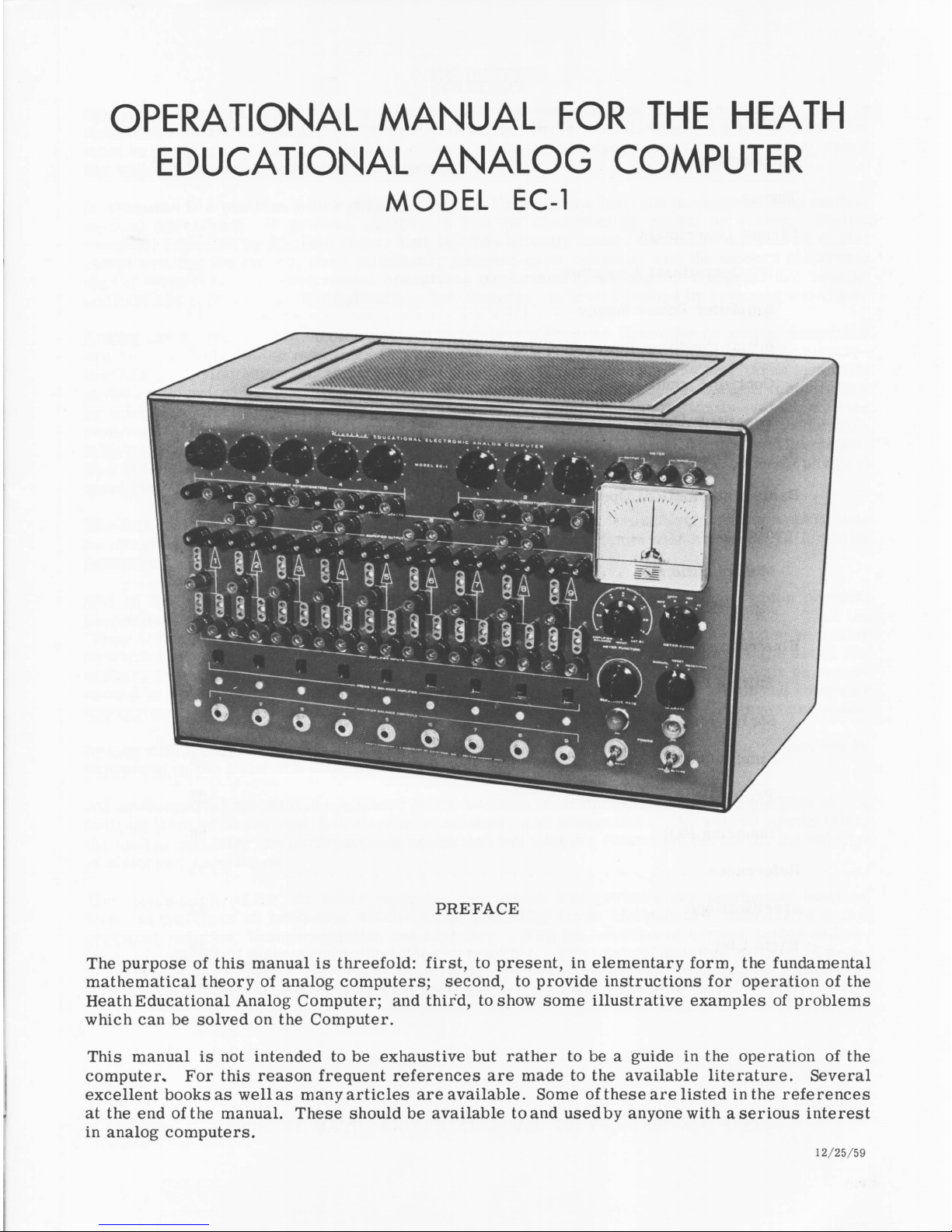
OPERATIONAL MANUAL FOR THE HEATH
EDUCATIONAL ANALOG COMPUTER
MODEL EC-1
PREFACE
The purpose of this manual is threefold: first, to present, in elementary form , the fundamental
mathematical theory of analog com puters; second, to provide instructions for operation of the
Heath Educational Analog Computer; and third, to show some illustrative examples of problems
which can be solved on the Computer.
This manual is not intended to be exhaustive but rather to be a guide in the operation of the
computer. For this reason frequent references are made to the available literature. Several
excellent books as well as many articles are available. Some of these are listed in the references
at the end of the manual. These should be available to and usedby anyone with a serious interest
in analog computers.
12/25/59

Preface
CONTENTS
1
Introdufction ....................................................................................................... 3
Theory .................................................................................................................. 4
Circuit Description
DC Operational Am plifier ....................................................................... 13
Am plifier Power Supply ........................................................................... 14
Initial Condition Power S u p p lie s ............................................................. 15
Control C i r c u i t ............................................................................................. 15
Repetitive O s c illa t o r .................................................................................. 15
General Operating I n s t r u c tio n s .................................................................... 16
Basic Mathematical Operations
A d d ition ............................................................................................................ 17
M u ltip lica tio n ................................................................................................ 19
Integration ....................................................................................................... 19
Illustrative Problems
Falling Body ................................................................................................ 21
Spring-M ass S y s t e m .......................... .• .................................................... 24
Simultaneous A lgebraic E q u a tio n s ......................................................... 26
P r o je c t ile ....................................................................................................... 27
Bouncing B a ll ....................................... 28
R e f e re n c e s ........................................................................................................... 31
S p e c i fi c a t io n s .................................................................................................... 32
Parts L i s t ........................................................................................................... 36
S c h e m a t ic .......................................... . 40
Page 2

INTRODUCTION
One of the wonders of the modern E lectronic Age is the computer or "Giant Brain", as it is
som etim es called. Actually, the computer is not a "B rain ” at all, since it does not think but
must be "told" what to do. It is capable of doing mathematical operations at much greater speed
and with greater accuracy than human beings.
A computer is a machine which perform s physical operations that can be described by mathe
matical operations. In general, computers may be classified as digital or analog. Digital
com puters operate by discrete steps, that is, they actually count. Common exam ples of digital
com puters are the abacus, desk calculator, punched-card machine, and the modern electron ic
digital computer. The fundamental operations perform ed by the digital computer are usually
addition and subtraction. Multiplication, for example, is accomplished by repeated additions.
Analog com puters operate continuously, that is, they measure. Examples of analog com puters
are the slide rule (which m easures lengths), the mechanical differential analyzer, the e le c tro
mechanical analog computer and the a ll-electron ic analog computer. The last three generally
measure electrical voltages or shaft rotations. Physical quantities such as weight, temperature
or area are represented by voltages. Voltage is the electrical analog of the variable being
analyzed. A rbitrary scale factors are set up to relate the voltages in the computer to the var
iables in the problem being solved. For example, 1 volt equals 5 feet or 10 volts equals 1 pound.
The name "analog" com es from the fact that the computer solves by analogy by using physical
quantities to represent numbers.
The fact that the analog computer operates continuously makes it very useful in such operations
as integration; for this reason com puters used this way are som etim es known as Differential
Analyzers.
One of the most powerful applications of analog com puters is simulation in which physical
properties, not easily varied, are represented by voltages which are easily varied. Thus the
"knee action" of an automobile front wheel suspension can be simulated on an analog computer
in which the weight of the automobile, the constant of the spring, the damping of the shock ab
sorb er, the nature of the road surface, the tire pressure and other conditions can be repre
sented by voltages. In practice these factors cannot be readily changed, but on the computer
any one or all of these may be varied at will and the results observed as the changes are made.
Analog com puters are especially useful in solving dynamic problems in which the motion can be
expressed in the form of a differential equation.
All mathematical operations necessary to the solution of ordinary differential equations can be
built up from addition, multiplication by a constant, and integration. * As will be shown later,
the analog computer can perform these operations and thus is a convenient device for the solution
of differential equations.
The combination of the six basic computer operations will perform any continuous function.
Some of the types of problem s which can be solved by these methods are radioactive decay,
chem ical reaction, beam oscillation and heat flow. With the addition of crystal diodes and r e 
lays, simulation of discontinuous functions is possible. This makes possible solution of prob
lem s involving saturation, backlash, hysteresis, friction, limit stops, vacuum tube character
istics, and different modes of operation such as sonic vs. subsonic flow.
* Shannon, C ., JOURNAL MATH. AND PHYSICS, Vol. 20, Pages 337-354, 1941.
Page 3

With the addition of special devices such as function generator and function multiplier, addi
tional operations may be perform ed such as multiplication of variables, computation of trig
onom etric, exponentional and logarithmic functions and generation of discontinuous functions. *
THEORY
In order to solve differential equations on an analog computer, it is necessary to have:
1. DC am plifiers (also called operational am plifiers) capable of performing the operation
of
a. Integration
b. Addition (or summation)
c. Multiplication by a constant
d. Multiplication by -l(in version )
2. A means of setting coefficients in a problem. This may be done by means of
a. Potentiometers
b. Changing the ratio of feedback resistance to input resistance.
3. A control system for starting and stopping solution of the problem , as well as resetting
the initial conditions so as to be ready for running a new solution with the same or new
coefficients and initial conditions.
The general procedure in solving a problem is to:
1. Set the machine variables (voltages) to the corre ct initial conditions.
2. Make the computing elements operative and force the voltages to vary in the manner
prescribed by the differential equations.
3. Observe and /or record the voltage variations, with respect to time, which constitute
the solution of the given problem .
4. Stop the machine and reset for a new run.
The heart of the analog computer is the DC operational am plifier which perform s the basic
mathematical operations necessary for the solution of problem s.
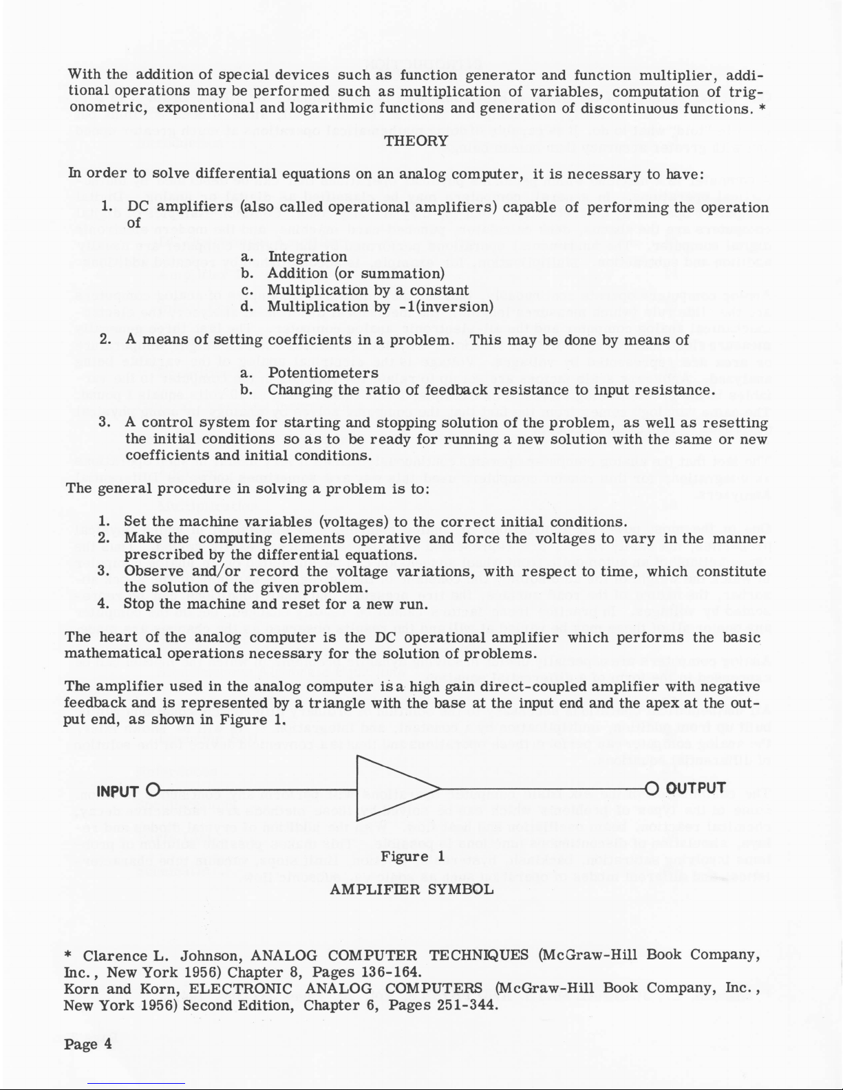
The am plifier used in the analog computer is a high gain direct-coupled amplifier with negative
feedback and is represented by a triangle with the base at the input end and the apex at the out
put end, as shown in Figure 1.
INPUT O - -O OUTPUT
Figure 1
AMPLIFIER SYMBOL
* Clarence L. Johnson, ANALOG COMPUTER TECHNIQUES (McGraw-Hill Book Company,
In c ., New Y ork 1956) Chapter 8, Pages 136-164.
Korn and Korn, ELECTRONIC ANALOG COMPUTERS (McGraw-Hill Book Company, In c .,
New York 1956) Second Edition, Chapter 6, Pages 251-344.
Page 4

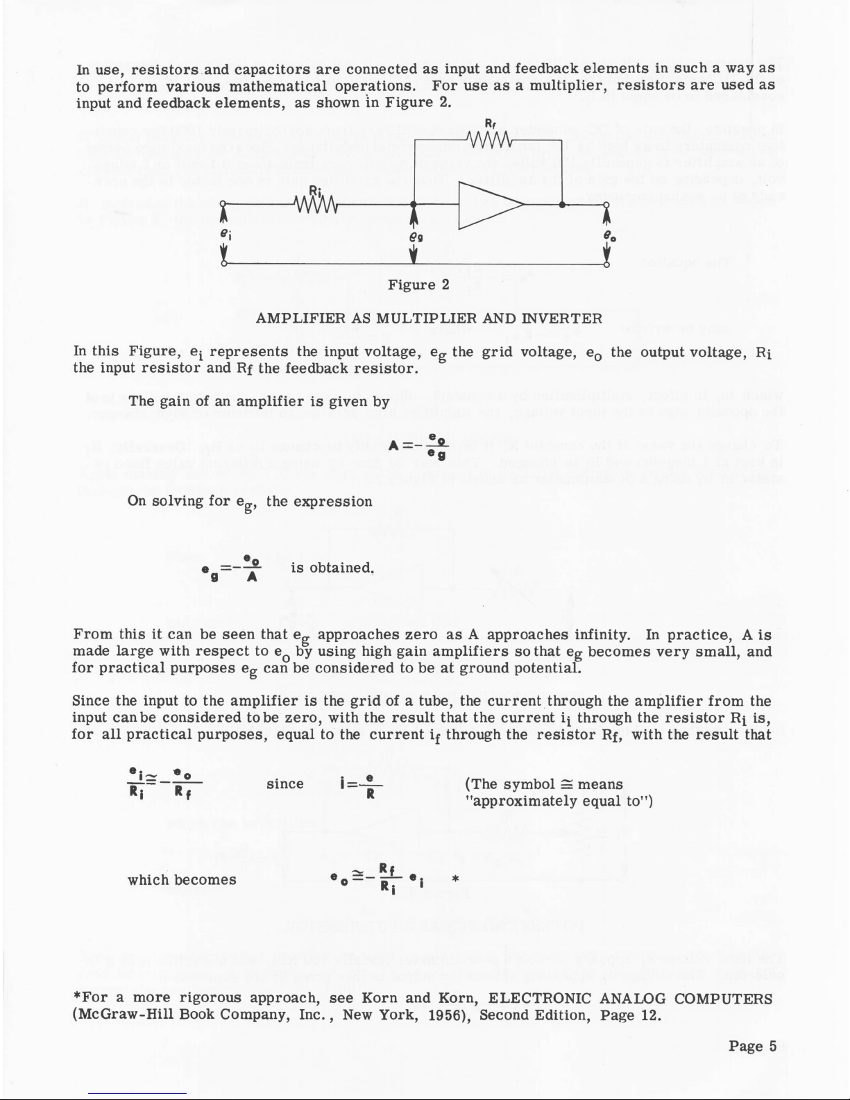
In use, resistors and capacitors are connected as input and feedback elements in such a way as
to perform various mathematical operations. For use as a multiplier, resistors are used as
input and feedback elements, as shown in Figure 2.
Rf
AMPLIFIER AS MULTIPLIER AND INVERTER
In this Figure, ei represents the input voltage, eg the grid voltage, e0 the output voltage, Ri
the input resistor and Rf the feedback re sisto r.
The gain of an amplifier is given by
On solving for eg, the expression
e = — . is obtained.
9 A
From this it can be seen that e g approaches zero as A approaches infinity. In practice, A is
made large with respect to eQ by using high gain am plifiers so that eg becom es very small, and
for practical purposes eg can be considered to be at ground potential.
Since the input to the amplifier is the grid of a tube, the current through the am plifier from the
input can be considered to be zero, with the result that the current if through the resistor Rf is,
fo r all practical purposes, equal to the current if through the resistor Rf, with the result that
* l ~ * o . e
-jp --—jj— since I — (The symbol = means
' * "approxim ately equal to")
2s Rf
which becom es eo — — # s
* i
♦For a more rigorous approach, see Korn and Korn, ELECTRONIC ANALOG COMPUTERS
(M cGraw-H ill Book Company, In c., New York, 1956), Second Edition, Page 12.
Page 5

The approximation which results from considering e = 0 w ill be used in the further discussion
of the DC am plifier but the "approximately equal to*' sign w ill not be used, that is, i^ w ill be
considered to be eqqal to if.
In practice, the gain of DC computer am plifiers will vary from approximately 1000 for repeti
tive computers to as high as 10° for a large com m ercial installation. Since the maximum output
of an am plifier is generally 100 volts, the value of eg w ill vary from about 0.1 volt to 1 m icro
volt, depending on the gain of the am plifier. Thus the am plifier gain is one factor in the accu
racy of an analog computer.
The equation eo5 l _ e .
may be written e_ — „ where
o - K .. K - —
which is, in effect, multiplication by a constant. Since, in most cases, the output voltage is of
the opposite sign to the input voltage, the am plifier also acts as an inverter or sign changer.
To change the value of the constant K, it is necessary only to change Rf or Rf. Generally, Rf
is kept at 1 megohm and Rj is changed. This may be done by using a different value fixed r e 
sistor or by using a potentiometer as shown in Figure 3.
POTENTIOMETER AS INPUT RESISTOR
Another method of obtaining odd constant values of Rj is shown in Figure 4.
POTENTIOMETER AS INPUT RESISTOR
The input voltage ef appears across a potentiometer (usually 100 Kfl), and a fraction p of it is
selected. The voltage e0 appearing a cro ss the output is then given by the expression
Page 6

Suppose, for example, a ratio of 3.7 is desired. If ji is made equal to 0.37 and R f/R f = 10
(Rf = 1 megohm and Rf = 100 Kfi), then eQ = -3.7 ej. Generally this method is to be preferred
over that shown in Figure 3.
In actual practice, the ratio R f/R f is generally greater than unity, since the am plifiers tend to
becom e unstable for values less than unity. Also the ratio R f/R f is 100 or less, as values
greater than 100 introduce inaccuracies in the solution of the problem .
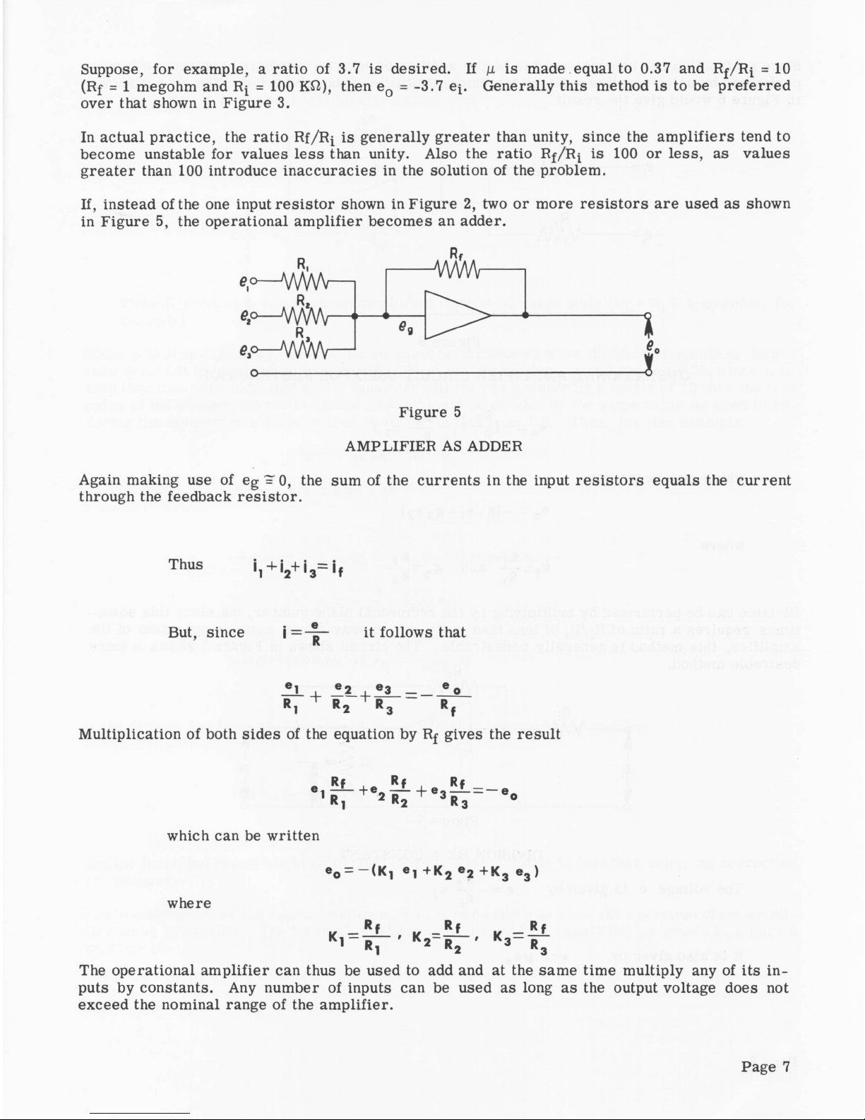
If, instead of the one input resistor shown in Figure 2, two or more resistors are used as shown
in Figure 5, the operational am plifier becom es an adder.
e°— VW W —
e , o - J W M r -
e , * - J WvW-
- M / W -
e0
i
Figure 5
AMPLIFIER AS ADDER
Again making use of eg = 0, the sum of the currents in the input resistors equals the current
through the feedback resistor.
ThUS i, + '2+ i3= 'f
But, since i = _ | r it follows that
—L . e 2 . e3 —
D + R* + R3
L1 " 2 " 3 - ' f
Multiplication of both sides of the equation by Rf gives the result
S t + . . * L = -
1
R, 2 R2 + ° 3R3
which can be written
e 0 — ( K , e , + K 2 e 2 +k e , )
Rf
K2=R-
where
= Rj_
[1 2 R2
The operational amplifier can thus be used to add and at the same time multiply any of its in
puts by constants. Any number of inputs can be used as long as the output voltage does not
exceed the nominal range of the amplifier.
Rf
K3= R 3
Page 7

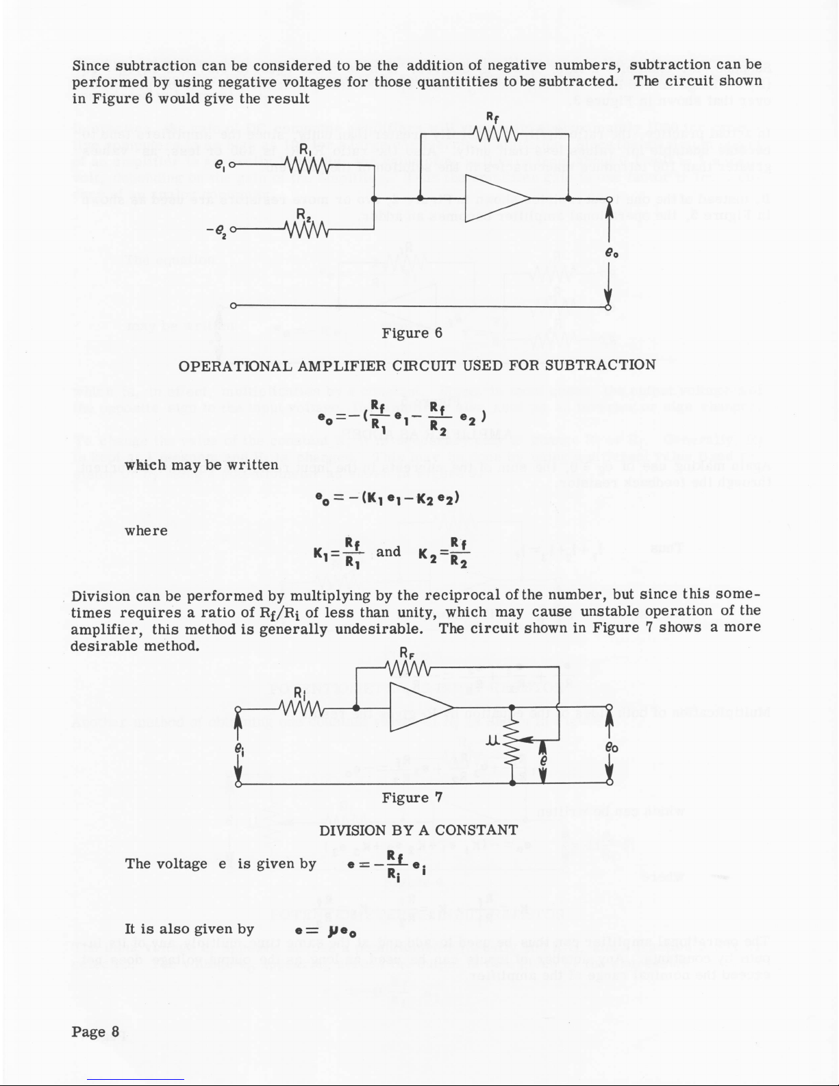
Since subtraction can be considered to be the addition of negative numbers, subtraction can be
perform ed by using negative voltages for those quantitities to be subtracted. The circuit shown
in Figure 6 would give the result
o -------------------------------------------------------------------------------- 1
Figure 6
OPERATIONAL AMPLIFIER CIRCUIT USED FOR SUBTRACTION
which may be written
where
- i t and Rf
K2 = r7
Division can be perform ed by multiplying by the recip rocal of the number, but since this som e
times requires a ratio of R f/R i of less than unity, which may cause unstable operation of the
am plifier, this method is generally undesirable. The circuit shown in Figure 7 shows a more
desirable method.
DIVISION BY A CONSTANT
The voltage e is given by
It is also given by e = p e 0
Page 8

where \i is the ratio of the voltage e0 appearing across the potentiometer to the voltage
across the arm of the potentiometer and ground.
R f
Thus p e_ = — - — e i
° R:
and e_ = — ®
Thus division by \i has been accom plished if R f/R f is made unity (Rf = Rf = 1 megohm, for
example).
Since p is less than unity, a scale factor must be introduced when dividing by numbers larger
than one. Let the desired divisor be 2.5. The value chosen for p. would then be 0.25, since p is
less than one. The indicated result (answer) w ill then be greater by a factor of 10 than the true
value of the answer, so the indicated answer must be divided by the same value as used in r e 
ducing the division to a value of less than one (in this case 10). Thus, for this example
®o 0.25 1 10 1 Rj "i
since 2.5 = 0.25 x 10
choosing Rj=r.= imeg, this becomes
1 / 1 x
eO - 0.25 *10' e i
which becom es 10 « 0 —~ q 25 *■
If the divisor had been 25, a factor of 100 would have been chosen, yielding
100 ®o o.25 *■
and the indicated result would be divided by 100. If the division is less than unity, no correction
is necessary.
Again making use of the approximation e „ = o, it is possible to show the operation of the am pli
fier as an integrator. The feedback resisto r is replaced by a capacitor, as shown in Figure 8
on Page 10.
Page 9

OPERATIONAL AMPLIFIER AS INTEGRATOR
e i _ ■_ dQ
Rj d t
Since dQ = efdeQ this becomes
Solving this equation for deQ gives the result
de0 =— ei<**
Rj cf
Integration of both sides gives
Where eiC is the constant of integration
(initial condition) and is the voltage
across the capacitor Cf at time t = o.
Thus the operational amplifier can integrate.
Figure 9
AMPLIFIER AS DIFFERENTIATOR
It is possible to show, by a sim ilar analysis, that the operational amplifier can be used to
differentiate. The amplifier is used very seldom for this purpose, however, since noise in the
input tends to be magnified by differentiation, whereas it tends to cancel out in integration.
Such circuits also tend to be unstable.
In p ractice, the value of the feedback resistor Rf, when used, is generally 1 megohm and the
value of the feedback capacitor C f, when used, is generally 1 pfd. The value of the input r e 
sistor usually varies from 0.1 megohm to 1.0 megohm, although in certain problems the values
may be different from these values.
Page 10

A combination of simple operations form s a complex operation. In general, an analog computer
is not used for addition alone or for multiplication by a constant as a single operation. These
can be better perform ed by other means. The value of the computer lies in its ability to combine
these simple operations into a com plex operation.
An example of a com plex operation is indicated by the circuit shown in Figure 10.
c
ei<>-
e'°— W W V n
-A/WVW
-AAM/V
-A/WW 1eo
J
Figure 10
COMPLEX OPERATION
This circuit solves the relationship
—l- r r ^ -
RC J L Rl e* ] dt + en (o)
where e0 (o) is the output voltage at time t = o (start of problem solution). Amplifier A is used
for sign inversion. It can be omitted if a minus result is acceptable.
Another example of a simple type of problem involving com plex operation is that of an object
falling due to the force of gravity. The acceleration which the body experiences is constant near
the surface of the earth and due to the force exerted on the object by the gravitational field of
the earth. This may be written as an equation,
d * y _
dt 2 -
where y is the distance the object falls in time t, and g is the acceleration given the object by
the earth's gravitational field. By integrating twice, it is possible to obtain an expression for y
in terms of g and the time t during which the body has fallen. This can easily be set up on the
computer, using two am plifiers as shown in Figure 11.
AMPLIFIER CONNECTIONS FOR SOLVING "FALLING BODY PROBLEM”
The input voltage e^ is supplied by a suitable power supply and the value of ei is chosen so that
eQ does not exceed the output capacity of amplifier 2. Instructions for setting up this problem
are given on Page 21. It is suggested, however, that the actual setup and solution of the prob
lem be withheld until the CIRCUIT DESCRIPTION and OPERATION sections of this manual have
been thoroughly reviewed and are generally understood.
Page 11

Other examples of the application of com plex operation to the solution of problems are given in
the section on OPERATION.
SCALE FACTORS
In the operation of the analog computer two factors must be considered. The first of these is
the amplitude factor. In general, the output of each am plifier must be kept within the range
±100 volts, the actual value depending on the am plifier used in the computer. In order to keep
the output within the specified lim its, it is generally necessary to scale down the input voltages.
It is not always possible to determine before hand the range of the voltages, in which case a
trial run can be made and after the voltages are observed, the proper amplitude scale factors
can be chosen. Sometimes it is possible to estimate the range of voltages from the physics of
the problem.
The other factor is time. If the product RiCf = 1 when Rf is measured in ohms and Cf is m eas
ured in farads, the computation is said to be in real time. This is so, for example, when Rf =
1 megohm and Cf = 1 jufd. (RiCf = 10® ohms x 10_® farad = 1) If the computer is operated such
that the solution is obtained in le ss time than is required for the physical solution to occur, the
operation is said to be faster than real time. This is very useful if the physical occurrence which
is being simulated requires considerable time. Tim e is also saved, permitting the solution of
more problem s in the same length of machine time.
Another advantage is that machine e rror is decreased, especially the e rror due to the leakage
resistance of the feedback capacitors. In general, the solution of a problem on the computer
should not require m ore than lto5 minutes. Longer solution tim es require special precautions.*
REPETITIVE OPERATION
It is desirable, for many problems, to repeat the solution and observe the effect on the solution
of changing the various param eters of the problem. This is made possible by repetitive oper
ation. Some means is provided for automatically resetting the computer and re-running the
problem. A cathode ray oscilloscope is convenient for observing the solution in this case.
Generally, one of the computer amplifiers is used to provide the sweep for the oscilloscope .
Details of operation will be discussed in the section on OPERATION.
ACCURACY
As was shown previously, the higher the am plifier gain the less will be the error in each com 
puting operation. Thus the accuracy depends in part on the gain of the operational amplifier.
A ccu racy also depends on the precision of the computing components, such as resistors and
capacitors. Time is also a factor in accuracy. In general, long runs introduce e rro rs due to
am plifier drift and capacitor leakage.
* Goode and Machol, SYSTEM ENGINEERING (McGraw-Hill Book Company, In c., New York,
1957), Pages 278-283.
Clarence L. Johnson, ANALOG COMPUTER TECHNIQUES (McGraw-Hill Book Company, In c .,
New York, 1956), Chapter 3, Pages 20-44.
Korn and Korn, ELECTRONIC ANALOG COMPUTERS (McGraw-Hill Book Company, Inc. ,
New York, 1956), Pages 30-35.
James B. Resnick, "Scale Factors for Analog Com puters", Product Engineering, M arch, 1954.
Page 12

Any variations in voltages in any part of the circuit of a direct-coupled amplifier cause va ri
ations in the output voltage which in turn introduce erro rs in the solution. With constant input
the output will vary, resulting in "d rift” , which increases with amplifier gain. This introduces
a paradox since, as has been shown, error is reduced by increasing amplifier gain but this in
turn increases drift which increases e rro rs. For this reason, very high gain am plifiers gener
ally use some means of stabilization in order to reduce drift. *
READ-OUT
For arithm etic problem s in which a single numerical answer is obtained, the result can be read
on the m eter. In problem s having a continuous solution (changing with time) an oscilloscop e is
desirable. It is possible in this case to watch the effect on the solution of varying the various
problem parameters. This is especially true when repetitive operation is used. In this case
one of the computer am plifiers is used to provide the sweep. The oscilloscop e must be a DC
scope.
If a permanent record of the solution is desired, a photograph of the o scilloscop e trace may be
made or a recording galvanometer may be used. Examples of both methods are shown in the
illustrative problem s.
NON-LINEAR OPERATION
A discussion of non-linear operation is beyond the scope of this manual. An excellent treatment
of non-linear operation can be found in ANALOG COMPUTER TECHNIQUES by Clarence L.
Johnson, Chapter 7, Pages 107-127.
CIRCUIT DESCRIPTION
DC OPERATIONAL AMPLIFIER
The general requirem ents for a DC am plifier for computer use are high gain, high input imped
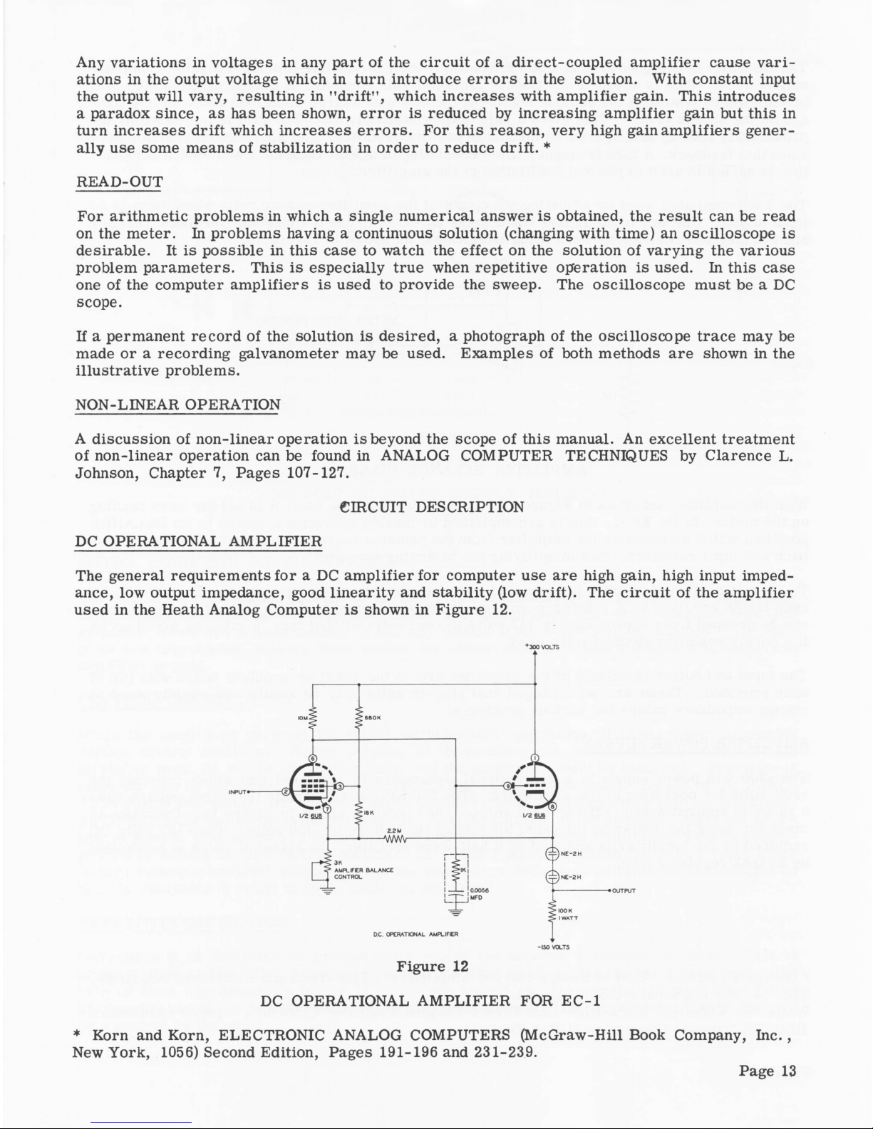
ance, low output impedance, good linearity and stability (low drift). The circuit of the amplifier
used in the Heath Analog Computer is shown in Figure 12.
+ 300 VOLTS
Figure 12
DC OPERATIONAL AMPLIFIER FOR EC-1
* Korn and Korn, ELECTRONIC ANALOG COMPUTERS (McGraw-Hill Book Company, Inc. ,
New York, 1056) Second Edition, Pages 191-196 and 231-239.
Page 13

The amplifier is designed around a6U8 tube with which it is possible to achieve a gain of approxi
mately 1000. This is adequate for the use for which this computer is designed. This high gain
is achieved by operating the pentode section of the 6U8 with a large plate load and with low volt
age on the screen grid. * This gives a gain of approximately 700. The gain is increased to ap
proxim ately 1000 by adding a small amount of positive feedback. The 2.2 megohm resistor p ro
vides this feedback. A high frequency filter consisting of a 1KS7 re sistor and a 5600 pjuf capac
itor in series is used to prevent oscillation of the amplifier.
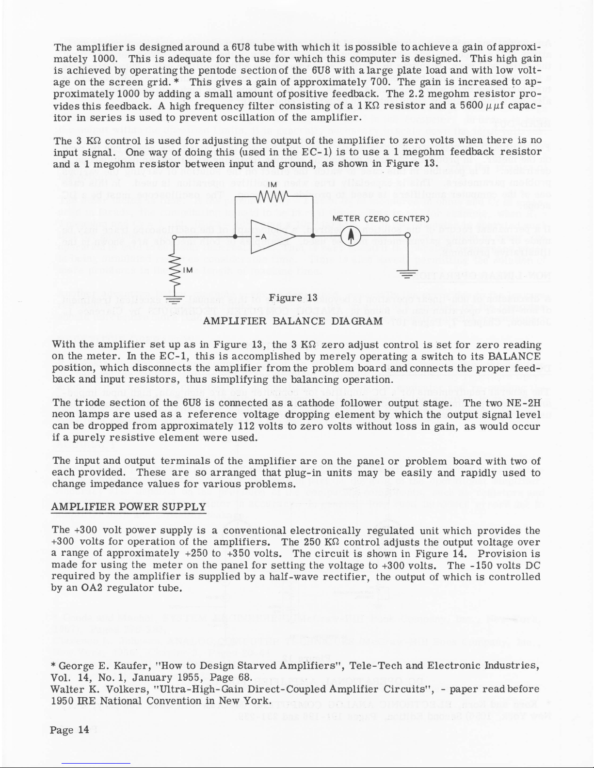
The 3 K£2 control is used for adjusting the output of the am plifier to zero volts when there is no
input signal. One way of doing this (used in the EC-1) is to use a 1 megohm feedback resistor
and a 1 megohm resistor between input and ground, as shown in Figure 13.
IM
With the am plifier set up as in Figure 13, the 3 Kf2 zero adjust control is set for zero reading
on the m eter. In the E C -1, this is accom plished by m erely operating a switch to its BALANCE
position, which disconnects the am plifier from the problem board and connects the proper feed
back and input resistors, thus sim plifying the balancing operation.
The triode section of the 6U8 is connected as a cathode follower output stage. The two NE-2H
neon lamps are used as a reference voltage dropping element by which the output signal level
can be dropped from approximately 112 volts to zero volts without loss in gain, as would occu r
if a purely resistive element were used.
The input and output terminals of the am plifier are on the panel or problem board with two of
each provided. These are so arranged that plug-in units may be easily and rapidly used to
change impedance values for various problem s.
AMPLIFIER POWER SUPPLY
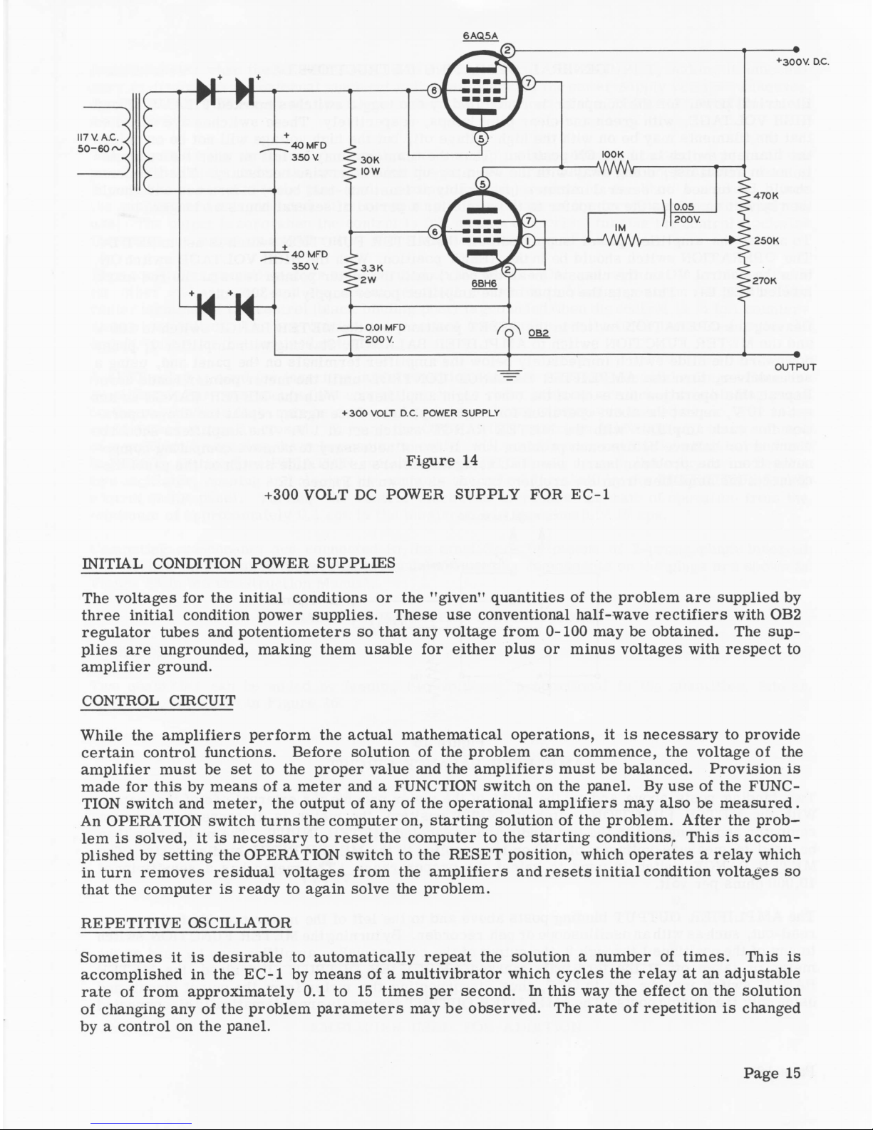
The +300 volt power supply is a conventional electronically regulated unit which provides the
+300 volts for operation of the am plifiers. The 250 K£7 control adjusts the output voltage over
a range of approximately +250 to +350 volts. The circuit is shown in Figure 14. P rovision is
made for using the m eter on the panel for setting the voltage to +300 volts. The -150 volts DC
required by the amplifier is supplied by a half-wave rectifier, the output of which is controlled
by an OA2 regulator tube.
* George E. Kaufer, "How to Design Starved A m p lifiers", T ele-T ech and E lectronic Industries,
Vol. 14, No. 1, January 1955, Page 68.
Walter K. Volkers, "Ultra-High-G ain D irect-Coupled Amplifier C ircuits", - paper read before
1950 IRE National Convention in New York.
Page 14

6AQ5A
O U T PU T
+ 3 0 0 V O LT D.C. PO W ER S U P P L Y
Figure 14
+300 VOLT DC POWER SUPPLY FOR EC-1
INITIAL CONDITION POWER SUPPLIES
The voltages for the initial conditions or the "given" quantities of the problem are supplied by
three initial condition power supplies. These use conventional half-wave rectifie rs with OB2
regulator tubes and potentiometers so that any voltage from 0-100 may be obtained. The sup
plies are ungrounded, making them usable for either plus or minus voltages with respect to
am plifier ground.
CONTROL CIRCUIT
While the am plifiers perform the actual mathematical operations, it is necessary to provide
certain control functions. Before solution of the problem can commence, the voltage o f the
am plifier must be set to the proper value and the am plifiers must be balanced. Provision is
made for this by means of a meter and a FUNCTION switch on the panel. By use of the FUNC
TION switch and m eter, the output of any of the operational am plifiers may also be m easured.
An OPERATION switch turns the computer on, starting solution of the problem. After the prob
lem is solved, it is n ecessary to reset the computer to the starting conditions. This is a ccom 
plished by setting the OPERATION switch to the RESET position, which operates a relay which
in turn rem oves residual voltages from the am plifiers and resets initial condition voltages so
that the computer is ready to again solve the problem.
REPETITIVE OSCILLATOR
Sometimes it is desirable to automatically repeat the solution a number of tim es. This is
accom plished in the E C -1 by means of a multivibrator which cycles the relay at an adjustable
rate of from approximately 0.1 to 15 tim es per second. In this way the effect on the solution
of changing any of the problem parameters may be observed. The rate o f repetition is changed
by a control on the panel.
Page 15

GENERAL OPERATING INSTRUCTIONS
E lectrical power for the computer is controlled by two toggle switches marked FILAMENT and
HIGH VOLTAGE, with green and clear pilot lamps, respectively. These switches are wired so
that the filaments may be on with the high voltage off, but the high voltage will not be on unless
the filament switch is in the ON position. Thus the filaments may be left on when the computer
is not in actual use, doing away with the warming-up time otherwise necessary. The filaments
should be turned on several minutes (preferably at least one-half hour) before use and should
then be left on unless the computer is to be idle for a period of several hours or longer.
To adjust the am plifier power supply output, the METER FUNCTION switch is set to SET B+.
The OPERATION switch should be in the RESET position. With the HIGH VOLTAGE switch ON,
turn the control VC on the chassis (near the rear) until the meter pointer rests at the red mark
labeled SET B+. This sets the output of the amplifier power supply to +300 volts.
Leaving the OPERATION switch in the RESET position, set the METER RANGE switch to 100 V
and the METER FUNCTION switch to AMPLIFIER BALANCE. Starting with am plifier 1, press
downward the slide switch immediately below the am plifier terminals on the panel and, using a
screw driver, turn the AMPLIFIER BALANCE CONTROL until the meter pointer reads zero.
Repeat this operation for each of the other eight am plifiers. With the METER RANGE switch
set at 10 V, repeat the above operation for each am plifier. Once again, repeat the above opera
tion for each amplifier with the METER RANGE switch set at 1 V. The amplifiers should be
checked for balance before each problem run. It is not necessary to rem ove computing com po
nents from the problem board when balancing amplifiers as the slide switch on the panel dis
connects the amplifier from the problem board, as shown in Figure 15.
TO P R O B LEM BOARD
i i
Figure 15
AMPLIFIER BALANCE CIRCUIT
Two binding posts above and to the right of the meter provide for external use of the meter.
With the METER FUNCTION switch in INPUT position, the meter is disconnected from the
computer and connected to the two binding posts labeled METER INPUT. The meter may then
be used to measure voltages of 100 or less applied to the METER INPUT binding posts. The
METER RANGE switch is used to select the proper range. The meter has a sensitivity of
10,000 ohms per volt.
The AMPLIFIER OUTPUT binding posts above and to the left of the meter provide for external
read-out, such as with an oscilloscop e or pen recorder. By turning the METER FUNCTION switch
to any of the positions 1 through 9, the output of the corresponding am plifier may be read on the
meter or taken off at the term inals marked AMPLIFIER OUTPUT. If desired, the METER
RANGE switch may be set to OFF, thus disconnecting the meter from the output circuit and
using only the binding posts. The AMPLIFIER OUTPUT terminals are automatically disconnected
Page 16

from the meter when the METER FUNCTION switch is at SET B+ or INPUT, making it unneces
sary to disconnect the external read-out unit when checking the power supply voltage. Likewise,
the METER INPUT term inals are disconnected atall positions of the METER FUNCTION switch
except INPUT.
The outputs of the three initial condition power supplies are connected to binding posts on the
panel immediately under the controls for the supplies. The outputs are not grounded, making
it possible to use either the plus (red) o r minus (black) terminal for the "hot" terminal. Since
the supplies are not grounded, it is necessary to ground one of the terminals of each supply in
use. The output is zero when the control is full counter clockw ise; turning the control clockw ise
increases the output up to 105 volts, with a maximum current of 5 ma.
Five coefficient potentiometers are provided on the panel. One end terminal is grounded, with
the other end terminal and the center terminal connected to binding posts on the panel. The
center terminal of the control (black binding post) is grounded when the control is in full counter
clockwise position. The ungrounded end terminal (red binding post) will be connected to the IC
supply voltage of the required potential.
A 4PST relay is used for inserting initial conditions and for rem oving residual voltages from the
am plifiers. For convenience, the connections to the relay contacts are brought to binding posts
on the panel where they may be connected a cross problem components as required. The relay
contacts are normally closed. Turning the OPERATION switch to MANUAL will start solution
of a problem by opening the relay contacts, which will remain open until the switch is returned
to RESET. Setting the OPERATION switch to REPETITIVE will connect the relay to the repeti
tive oscillator, opening and closing the contacts at a rate determined by the REPETITION RATE
control on the panel. Turning the control clockwise increases the rate of operation from the
minimum of approximately 0.1 cps to the maximum of approximately 15 cps.
Computing components are connected to the amplifiers by means of 2-prong plugs inserted
into sockets on the panel. Suggested methods of mounting components on the plugs are shown in
Figure 25 in the Construction Manual.
BASIC MATHEMATICAL OPERATIONS
ADDITION
Two quantities can be added by feeding two voltages, proportional to the quantities, into an
am plifier, as shown in Figure 16.
Figure 16
AMPLIFIER USED FOR ADDITION
Page 17

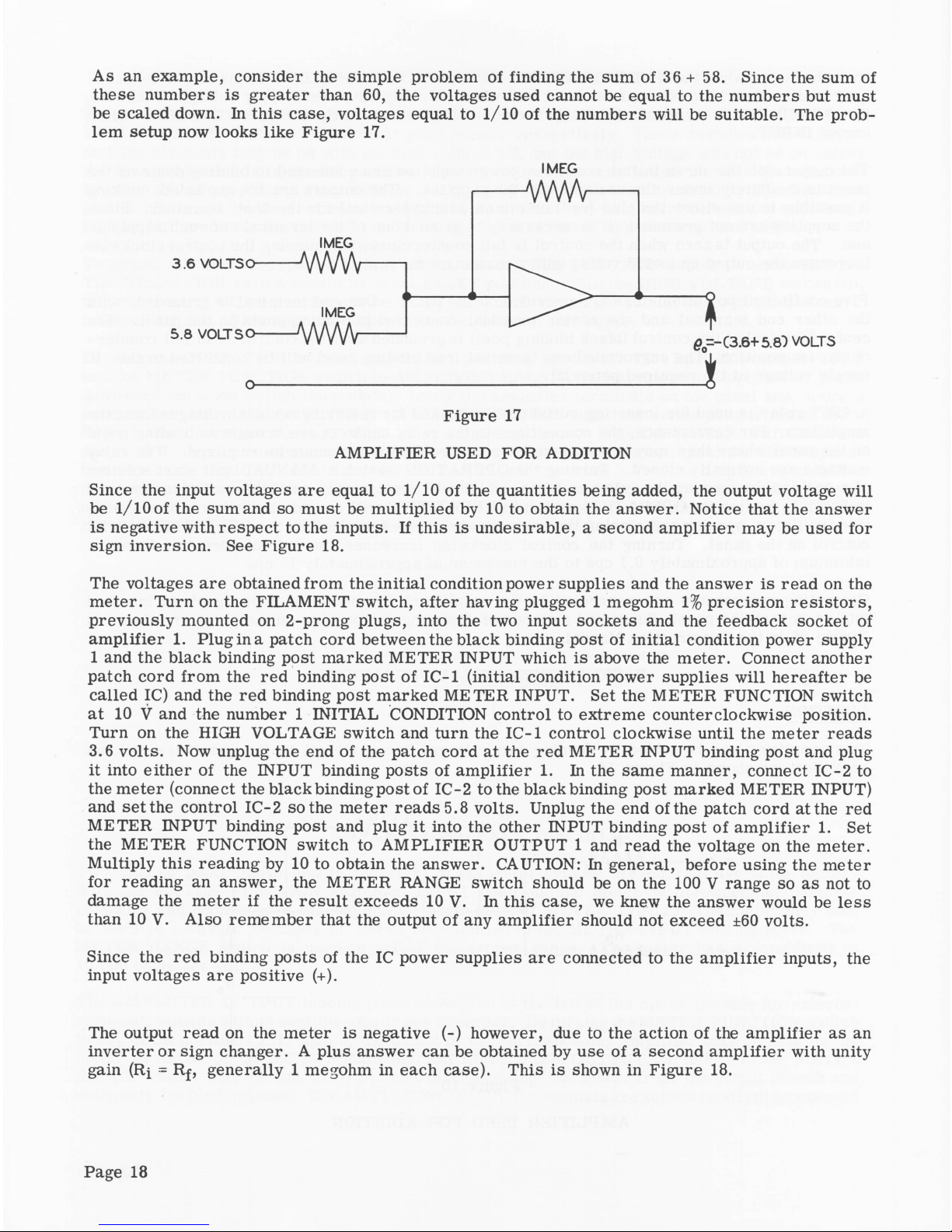
As an example, consider the simple problem of finding the sum of 36 + 58. Since the sum of
these numbers is greater than 60, the voltages used cannot be equal to the numbers but must
be scaled down. In this case, voltages equal to 1/10 of the numbers will be suitable. The prob
lem setup now looks like Figure 17.
I MEG
AMPLIFIER USED FOR ADDITION
Since the input voltages are equal to 1/10 of the quantities being added, the output voltage will
be 1 /lO o f the sum and so must be multiplied by 10 to obtain the answer. Notice that the answer
is negative with respect to the inputs. If this is undesirable, a second amplifier may be used for
sign inversion. See Figure 18.
The voltages are obtained from the initial condition power supplies and the answer is read on the
meter. Turn on the FILAMENT switch, after having plugged 1 megohm 1% p recision resistors,
previously mounted on 2-prong plugs, into the two input sockets and the feedback socket of
am plifier 1. Plug in a patch cord between the black binding post of initial condition power supply
1 and the black binding post marked METER INPUT which is above the m eter. Connect another
patch cord from the red binding post of IC-1 (initial condition power supplies will hereafter be
called IC) and the red binding post marked METER INPUT. Set the METER FUNCTION switch
at 10 V and the number 1 INITIAL CONDITION control to extrem e counterclockwise position.
Turn on the HIGH VOLTAGE switch and turn the IC-1 control clockw ise until the m eter reads
3.6 volts. Now unplug the end of the patch cord at the red METER INPUT binding post and plug
it into either of the INPUT binding posts of amplifier 1. In the same manner, connect IC-2 to
the meter (connect the black binding post of IC-2 to the black binding post marked METER INPUT)
and set the control IC-2 so the meter reads 5.8 volts. Unplug the end of the patch cord at the red
METER INPUT binding post and plug it into the other INPUT binding post of am plifier 1. Set
the METER FUNCTION switch to AMPLIFIER OUTPUT 1 and read the voltage on the meter.
Multiply this reading by 10 to obtain the answer. CAUTION: In general, before using the meter
for reading an answer, the METER RANGE switch should be on the 100 V range so as not to
damage the meter if the result exceeds 10 V. In this case, we knew the answer would be less
than 10 V. Also rem ember that the output of any amplifier should not exceed ±60 volts.
Since the red binding posts of the IC power supplies are connected to the am plifier inputs, the
input voltages are positive (+).
The output read on the meter is negative (-) however, due to the action of the amplifier as an
inverter or sign changer. A plus answer can be obtained by use of a second amplifier with unity
gain (Ri = Rf, generally 1 megohm in each case). This is shown in Figure 18.
Page 18