Luzchem SPR-02 User manual

Spectroradiometers
Instruction manual
SPR-01 and SPR-02
Version 2.3
August 2004
© Copyright Luzchem Research, Inc.

2
Table of Contents
1. Initial set-up ......................................................................................................... 3
1.1. Model SPR-01............................................................................................. 3
1.2. Model SPR-02............................................................................................. 3
2. Understand your hardware................................................................................... 4
2.1. Detector head.............................................................................................. 4
2.2. Spectrometer............................................................................................... 5
2.3. Fiber optic cable.......................................................................................... 5
2.4. Attenuator ................................................................................................... 6
2.5. Verification lamp (model SPR-01 only)..................................................... 6
3. Software Instruction manual................................................................................ 8
3.1 General........................................................................................................ 8
3.2 Software Installation................................................................................... 8
3.3 Starting the software................................................................................... 9
3.4 Optimize Integration Time.......................................................................... 9
3.5 Power/Intensity Spectra............................................................................ 10
3.6 Data reliability evaluation......................................................................... 12
3.7 Timed Acquisition .................................................................................... 13
3.8 File Formats.............................................................................................. 15
4. Help ................................................................................................................... 18

3
1. Initial set-up
1.1. Model SPR-01
The Spectroradiometer model SPR-01 consists of three parts:
•The control module and detection fiber
•The detection head (light integrating module)
•A USB cable
Assemble the instrument as indicated below. The connection of the blue fiber optic
cable to the detector should be ‘finger tight’. Do not use any tools and do not force.
The calibration parameters for your instrument have been determined with the same
components with which it was supplied. Individual parts are not interchangeable.
Place detector in
Corner for verification
Spectroradiometer
SPR-01- 235-850 nm
Detector
Optical fiber
Control Module
USB cable
Verification
lamp
Figure 1.1: Schematic diagram for SPR-01
Optical fibers are fragile and cannot be bent at any angle. The minimum momentary
bent radius is 60 mm, and the minimum long term bent radius is 100 mm (4 inches).
Assemble your instrument as indicated above, and connect the USB cable to an
available port in your computer. Software installation is explained in Section 3 of
this manual.
1.2. Model SPR-02
The Spectroradiometer model SPR-02 consists of two parts:
•The control module that with its built-in detection head (light integrating
module)
•A USB cable
SPR-02 is sold fully assembled. Only the USB cable needs to be installed and
connected to the computer. Software installation is explained in Section 3 of this
manual.

4
Figure 1.2: Spectroradiometer models SPR-01 (left) and SPR-02
2. Understand your hardware
2.1. Detector head
Figure 2.1 shows the assembly of the detector head or light integrator. The detector is
constructed of PTFE encased in light scattering aluminum and has been designed for
maximum efficiency in a low-profile integrator.
Figure 2.1: Assembly of the detector head

5
The top of the integrator has a solid cover that can be used when monitoring the dark
background. We have found it convenient to leave one holding screw loosely in
place and simply rotate the cover to monitor dark and light signals, see Figure 2.2.
Figure 2.2: Closed and open detector assembly, as used in Model SPR-01
It is important that you do not allow dust or other materials to fall inside the detector
head; this would invalidate the calibration provided by Luzchem.
The bottom of the detector head has a threaded hole (1//4-20 threads) that can be used
for mounting the detector. A very thin aluminum plate protects the PTFE
compartment from damage by objects inserted through the mounting hole. The
maximum penetration is 3 mm. Do not force screws to penetrate more than this, since
they can damage the integrator compartment.
2.2. Spectrometer
The heart of Luzchem spectroradiometers is a 2048 element spectrometer contained
in the control module. It covers a minimum range of 230 to 860 nm and has optical
components to optimize ultraviolet detection. Data points are acquired about every
~0.3 nm; however the software converts the data so that points are displayed at 1 nm
intervals.
The spectrometer is quite robust and ideal for field work and wherever portability is
important. However, it should be protected for water and high temperatures.
Stray light is quite low, for example: < 0.05% at 600 nm, < 0.10% at 435 nm, and <
0.10% at 250 nm. The grating used has 600 lines/mm and has been blazed at 400 nm.
Spectrometer control is achieved via the USB port; no other source of power is
required to operate the spectrometer.
2.3. Fiber optic cable
The fiber optic cable, connecting the spectrometer to the detector head is an integral
part of your instrument (it is fully enclosed in the spectroradiometer model SPR-02),
and instrument calibration is dependent on the fiber used.

6
The fibers used are terminated with SMA connectors that have been carefully
polished to achieve adequate optical performance. Luzchem uses high-OH fibers to
optimize ultraviolet performance. For model SPR-01 the fiber used is 300 µm in
diameter. The minimum allowed momentary radius is 60 mm (~2.5 inches), and the
minimum long term radius is 100 mm (4 inches). Bending the fiber beyond these
limits can cause permanent damage that also invalidates the calibration factors. Fiber
replacement requires recalibration of the instrument.
Instructions for SPR-01 only
When installing the fiber, the connection should be “finger tight”. Do not use tools
for this purpose.
The female SMA connector on the detector head should not move when installing or
disconnecting the fiber. It has been installed with a special adhesive that under
normal force conditions will prevent the female connector on the detector head from
moving. If this connector moves it will be necessary to reinstall it matching exactly
the calibration distance. Contact Luzchem for assistance.
2.4. Attenuator
Luzchem spectroradiometers are supplied with a PTFE film attenuator that reduces
the light input by about one order of magnitude. A generic transmission curve is
supplied with all attenuators.
Luzchem can perform a custom NIST traceable calibration for the attenuator supplied
with the system. For many applications the attenuator is not essential; however, for
some solar and sunbed applications, the attenuator may be useful to increase the
dynamic range of the instrument.
2.5. Verification lamp (model SPR-01 only)
Model SPR-01 includes a low pressure mercury lamp that operates with 4 AA
batteries. The lamp is controlled by a switch at the back of the instrument. This
switch does not need to be on to operate the radiometer, but only to use the
verification lamp. The verification lamp has the spectrum of Figure 2.3 (this is a
power spectrum), with a characteristic band at 254 nm that should be within ±1 nm of
the wavelength read.

7
0
10
20
30
40
50
60
300 400 500 600 700 800
Power (mWm-2nm-1)
Wavelength, nm
254 nm
Figure 2.3. Power spectrum for the verification lamp.
The correct positioning of the detector on the verification lamp is illustrated in Figure
2.4. In addition to verification of the wavelength, the verification lamp is useful in
determining the integrity of the optical fiber. Typically the intensity (that is, before
conversion to a power spectrum) should be between and 50 and 150 counts at 254 nm
for an integration time of 1000 ms.
Figure 2.4. Positioning of the detector head on the verification lamp.
If the counts at 254 nm are significantly less than 50, change the batteries (alkaline
batteries are recommended). If the problem is not resolved by this, it could be an
indication of a ruptured fiber; in this case, contact Luzchem for advice. Lamp usage
for verification purposes normally does not exceed a few minutes, and batteries last
about 12 hours of actual usage. Figure 2.5 shows a representative discharge curve
under continuous operation.

8
0
10
20
30
40
0 10000 20000 30000 40000
Power (mWm-2nm-1)
Time, seconds
Verification lamp discharge
monitored at 254 nm
Figure 2.5. Verification lamp discharge curve monitored at 254 nm.
3. Software Instruction manual
3.1 General
The purpose of this Section is to provide training on the acquisition and viewing of
spectra. This application can acquire information at timed intervals ranging from
1/10 of a second to hours. In order to establish the best possible integration time, the
spectroradiometer application is equipped with an “Optimize Integration Time”
function. This function searches for the best integration time for the intensity of the
incident light.
In order for the spectroradiometer application to be able to acquire data, it needs to be
connected to the spectroradiometer instrumentation. However, it can be used
independently to view previously acquired files. The application also requires that
the LabVIEW run time engine be loaded in the computer in use. The LabVIEW run
time engine is provided in the installation package.
3.2 Software Installation
3.2.1 On a computer already having the spectrometer driver: You may
already have a driver installed for the hardware. If this is the case, all you
need to do is install the application. Insert the CD into the CD-ROM
drive. A setup application should automatically appear. If it does not,
locate the folder named Spectroradiometer v2.2, open the “Installer”
folder, and install the application. The setup application will install both
the LabVIEW run time engine as well as the application. Once the
installation is complete you may need to restart your computer.
3.2.2 On a computer with no spectrometer driver: In this case you need to
install both the application, and driver for the hardware.Modern
operating systems such as Win XP will automatically detect new hardware
and search for an appropriate driver. The driver for the hardware is

9
located on the CD provided. On older operating systems, the user has to
initiate the installation of the driver:
3.2.2.1 Navigate to the Start>Settings>Control Panel>Add New Hardware
3.2.2.2 Follow the instructions on the screen
3.2.2.3 Insert the Luzchem CD, and the operating system will find and install
the appropriate driver
3.2.2.4 To install the application follow the directions in part a.
3.3 Starting the software
To start the spectroradiometer application, double click the shortcut on the desktop, or
the actual application in the Program Files folder. Please note that the application is
only compatible with the spectrometers sold by Luzchem. If the software does not
recognize the spectrometer, it will give an error message and close.
3.4 Optimize Integration Time
The optimize integration time function tests the intensity of the light and searches for
an appropriate integration time. This function is important because if the integration
time is too short, the data is susceptible to errors introduced by noise. If the
integration time is too long, the spectrometer can saturate, and the data above the
saturation point will be a flat line. The spectrometer saturation level is 4000 counts.
3.4.1 Navigate to the “Start Optimize Integration” tab
3.4.2 Press the “Start Optimize” button
3.4.3 Turn on the light and press “Go”. Note that the optimize function does not
require a dark measurement.
3.4.4 The application will test different integration times in order to find the best
one. Once the optimization is done, a dialog box will inform the user of
the optimized integration time. If the integration time is less than 10 or
greater than 1000, a warning message will appear. Please note that the
threshold for the spectrometer is 10 ms. An integration time lower than 10
ms will result in inaccurate readings.
3.4.5 If the optimized integration time falls in an acceptable range, all
integration times in the program will be set to this value. If the optimized
integration time is less than 10, the integration times will remain the same,
and if it is greater than 1000, the integration times will be set to 1000. The
user can override these values.
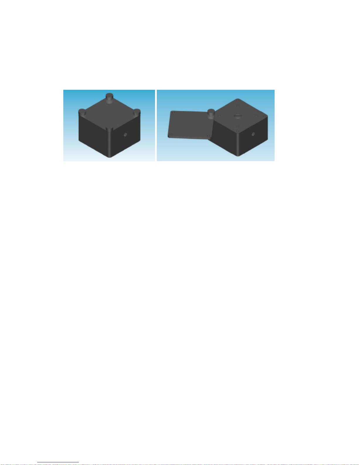
3.4.6 If the signal saturates at 10 ms integration time the use of an attenuator is
highly recommended (See section 2.4).

10
3.5 Power/Intensity Spectra
Power or intensity spectra can be acquired alone, or extracted from a timed
acquisition file. This section will cover acquiring a spectrum by itself.
Definitions: An intensity spectrum is a plot of counts against wavelength;
it shows the raw data acquired by the detector; it does not use
energy units. A power spectrum shows the energy distribution
as a function of wavelength; the Luzchem system displays this
in units of mW m
-2nm-1. An intensity spectrum can be
converted to a power spectrum by using a calibration file.
3.5.1 If desired, optimize integration time by following steps above.
3.5.2 Navigate to the “Spectroradiometer” tab.
3.5.3 Acquire a dark reference by turning off the source lamp or by blocking the
light input.
3.5.4 Open the light input window and acquire a sample.
3.5.5 Note that the data that is viewed on the acquisition graph can be changed
by using the radio buttons beneath the graph:
Figure 3.1: Radio buttons select the sets of data displayed
3.5.6 To create a power spectrum from the desired data, an appropriate
calibration file must be chosen. To use Luzchem’s calibration file, check
the box labeled “Use Luzchem’s supplied calibration”
3.5.7 To use your own calibration file, make sure the Luzchem’s supplied
calibration box is not checked and then press the “Browse” button or type
in the path to the calibration file:
Figure 3.2: Selection of a calibration file other than the Luzchem file built into the
control software.
3.5.8 The calibration file must be a per-millisecond text file with the following
format:
•Line 1: “Calibration Merge File”
•Line 2-4: Information you wish to save
•Line 5: Minimum Wavelength (tab) Maximum Wavelength
•Line 6 –11: Information you wish to save
•Line 12: Wavelength w1 (tab) Calibration at w1

11
•Line 13…:Wavelength w2 (tab) Calibration at w2
•A one nm wavelength interval is required. Also, a calibration wavelength
should exist for each wavelength in the acquisition. If a desired wavelength
does not exist in the calibration file, the resulting waveform will produce a
zero at that wavelength.
3.5.9 Once the calibration file has been chosen press the “Power Spectra”
button. A power spectrum will then appear on the Display graph. On the
left is the power (mW/m2) in the UVA, UVB, UVC, Visible, and user-
selected spectrum (Figure 3.3). These spectra can be viewed on the
display graph by checking the radio buttons to the left of the numbers
(Figure 3.4).
Figure 3.3: Definition of a customer-selected integration range
Figure 3.4: Shaded display of a selected integration range.
3.5.10 Intensity spectra can be created using the “Intensity Spectra” button. This
will transfer the data from the acquisition graph to the display graph where
it can be saved. UVA, UVB, UVC, and Visible spectra cannot be viewed
on the intensity graph.
3.5.11 To save the spectrum press the “Save Spectra” button located below the
graph. This will save the graph in a tab delimited text file that can easily

12
be opened with most spreadsheet and graphing applications. (Please see
the “File Format” section for the formatting of the intensity/power file.)
3.5.12 Once the spectrum is saved it can be opened at any time by using the
“Read File” button. An intensity spectrum can be opened and converted
to a power spectrum. In this case it is essential to use the calibration file
applicable at the time of acquisition.
3.6 Data reliability evaluation
A switch on the left lower main screen allows this option to be turned on and off.
The default as the program starts is ON. Figure 3.5 shows this control.
Figure 3.5: Data reliability evaluation turned on. Note ‘gray’ values when the
criterion set in the optimize tab is not met.
The data are shown in grey when they do not meet the significance criterion set in
the optimize tab. If should be noted that Luzchem sets a very high standard as a
default; users should set values that meet their own requirements. This is done in
the “Optimize” tab, where you will find in the left region the menu of Figure 3.6.
You have three options:
•An ON/OFF switch serves the same function as that on the main
window.
•The percent of the data that must meet the criterion.
•The number of counts below which the data is judged unreliable.
Note that when the data is labeled as unreliable, it only means that the
numeric value posted in the front window may have considerable error;
however, in general it is a good assumption that for practical purposes the
value is very small or zero.
In regions where there is essentially no light, one expects points with very
small values showing a random distribution around zero; i.e., 50% of the
values could be negative. This is normal. To improve the data increase

13
the number of averages, and ensure that the dark measurement totally
prevents light from reaching the detector.
In the UVC region it is possible that some light sources or materials
eliminate all light at the short wavelength range, such as wavelengths
below 250 nm. While the instrument range is 235 to 850 nm, you may
want to reduce the range to one that is more appropriate to your own light
sources. You can do this in the main screen.
Figure 3.6: Data reliability evaluation turned on. Two controls set the criterion
for data evaluation.
3.7 Timed Acquisition
The timed acquisition tab is very useful if you wish to see how the intensity of a lamp
or light source changes over time. It is very important to check your power
management options before performing a timed acquisition that will be left alone for
long periods of time. To turn off standby or hibernation :
•Navigate to Start>Settings> Control Panel
•Click on the Power Management icon
•Set system standby to “Never”

14
•Set hibernation to “Never” – Please be aware that some operating system will
not have a hibernation option.
•Click “Apply” and/or “OK” to save the settings and exit the power management
window.
To perform a timed acquisition:
3.7.1 If desired, optimize the integration time by following the steps outlined in
the Optimize Integration Time section. Note that the detector will saturate
if the intensity increases by more than 60% during the timed acquisition.
Use a shorter integration time if this is likely.
3.7.2 Press on the “Timed Acquisition” tab
3.7.3 Set the acquisition interval and total acquisition time (see Figure 3.7).
Figure 3.7: Selection of parameters for a timed acquisition
3.7.4 The Total acquisition time must be greater than or equal to the acquisition
interval. If this condition is not satisfied, an error message will appear and
the acquisition will be cancelled (Figure 3.8).
Figure 3.8: Error message following selection of incompatible parameters for
a timed acquisition.
3.7.5 If (integration time + transmission delay)*number of samples is greater
than the acquisition interval, an error will occur. In this case, either the
integration time or the number of samples to average must be decreased so
that (integration time + transmission delay)*number of samples is less that
the acquisition interval. Transmission delay is approximately 12 ms.
3.7.6 The acquisition interval can be as low as 0.1 seconds. Any lower and an
error message will appear.
3.7.7 When all parameters are set, press the “Start Timed Acquisition” button.
Acquisition interval
Total acquisition time

15
3.7.8 If the acquisition interval is less than 1 second, the top graph will not be
updated as the acquisition occurs. This is to save processor resources.
However, if the interval is greater than or equal to one second, the top
graph will be updated at each acquisition. The current time can be viewed
in the box in the bottom left hand side of the graph.
3.7.9 If the acquisition interval is equal to or greater than 10 seconds, a timer
will appear in the bottom left of the graph, counting down the seconds to
the next acquisition.
3.7.10 The acquisition can be stopped at any time by pressing the “Stop Timed
Acquisition” button.
3.7.11 When the acquisition is finished, a dialog box will appear and ask you
whether you would like to save the current timed acquisition. If you wish
to save, press yes, if you do not wish to save, press no. The acquisition
can be saved later. Timed acquisition files can be quite large and may
take a few seconds to load and save.
3.7.12 In order to extract a kinetic trace, choose a wavelength on the bottom left-
hand side of the screen. Next, press “Save Kinetic Trace”. The line of
information will be saved with the file.
3.7.13 In order to extract a spectrum from the timed acquisition, choose the time
at which you wish to extract the spectrum. Next, press “Save Spectrum”.
The line of information will be saved with the file. The file will also be
transferred to the “Spectroradiometer” tab where it can be edited and
manipulated.
3.7.14 The entire timed acquisition can be converted to a power file. This can be
done by choosing an appropriate calibration file. (Either Luzchem’s
supplied calibration, or a user calibration file.) Next, press the “Convert to
Power” button to calibrate all of the data.
3.7.15 For file formats please see the “File Formats” section.
3.8 File Formats
The spectroradiometer saves four types of files: spectrum files, timed acquisition
files, kinetic traces, and spectrum files extracted from a timed acquisition. Below is a
summary of the information contained in each file:
3.8.1 Spectrum/Power File:
Line 1 “Spectroradiometer” (tab) “Intensity” / “Power” (depending on spectrum
type saved)
Line 2 Integration time (tab) Samples to average
Line3 Minimum wavelength (tab) Maximum wavelength
Line 4 Line of information

16
Line 5 Serial number of spectrometer
Line 6-9
Line 10 “Wavelength” (tab) “Intensity” (tab) “Power”
Line 11 Wavelength w1 (tab) Intensity data at w1 (tab) Power data at w1 (if
applicable)
Line 12… Wavelength w2 (tab) Intensity data at w2 (tab) Power data at w2 (if
applicable)
In an intensity file the column for ‘power data’ will be blank.
3.8.2 Timed acquisition file:
Line 1 “Spectroradiometer –Timed Acquisition”
Line2 “Intensity” / “Power”
Line 3 Integration time (tab) Samples to Average
Line 4 Minimum wavelength (tab) Maximum wavelength
Line 5 Line of information
Line 6 Serial number of spectrometer
Line 7-9
Line 10 Wavelength array separated by tabs
Line 11 Time array separated by tabs
Line 12 Spectrum at time t1 separated by tabs
Line 13… Spectrum at time t2 separated by tabs
3.8.3 Kinetic Trace:
Line 1 “Spectroradiometer –Kinetic”
Line 2 Wavelength at which the kinetic trace was taken
Line 3 Line of information
Line 4 Serial number of spectrometer
Line 4 Time per point (sec)
Line 6-11
Line 12 “Time” (tab) “Power” / “Intensity”
Line 13 Time t1 (tab) power/intensity at t1
Line 14… Time t2 (tab) power/intensity at t2
3.8.4 Spectrum extracted from timed acquisition:
Line 1 “Spectroradiometer -Spectrum” (tab) “Intensity” / “Power” (depending on
the type of spectrum saved)
Line 2 Integration time (tab) Samples to average
Line 3 Minimum wavelength (tab) Maximum wavelength
Line 4 Line of information
Line 5 Serial number of spectrometer
Line 6-8

17
Line 10 “Spectrum at time:” time at which spectrum was extracted
Line 11 “Wavelength” (tab) “Intensity” (tab) “Power”
Line 12 Wavelength w1 (tab) Intensity at w1 (tab) Power at w1 (if applicable)
Line 13… Wavelength w2 (tab) Intensity at w2 (tab) Power at w2 (if applicable)

18
4.Help
To access the in-program help, click on the “Help” button, or navigate to Help >
Topic Help on the menu bar.