AFM Workshop LS-AFM User manual

LS-AFM
Users Guide
V 1.1
Part # 10-1121-16

Denitions and Symbols
The following terms and symbols are used in this document and also appear on the product
where safety-related issues occur.
General Warning or Caution
The exclamation symbol may appear in warning and caution tables in this document. This
symbol designates an area where personal injury or damage to the equipment is possible.
European Union CE Mark
The presence of the CE Mark on AFM Workshop equipment means that it has been
designed, tested and certied as complying with all applicable European Union (CE) regula-
tions and recommendations.
Warnings/Cautions/Notes
The following are denitions of the warnings, cautions and notes that may be used in this
manual to call aLSention to important information regarding personal safety, safety and
preservation of the equipment, or important tips.
WARNING
Situation has the potential to cause bodily harm or death.
CAUTION
Situation has the potential to cause damage to property or
equipment.
NOTE
Additional information the user or operator should consider.

Contents
1. Introduction to Atomic Force Microscopy..................................................................1-1
2. Introduction to the LS-AFM.........................................................................................2-1
2.1. Computer...................................................................................................2-1
2.2. Stage..........................................................................................................2-1
2.3. Ebox..........................................................................................................2-2
2.4. Video Optical Microscope.........................................................................2-2
2.4.1 Top View Video Optical Microscope.....................................2-2
2.4.2 Inverted Optical Microscope.................................................2-2
3. Software..........................................................................................................................3-1
3.1. Installation Procedure...............................................................................3-1
3.1.1. Gwyddion Image Analysis Software......................................3-1
3.2. AFM-View Software....................................................................................3-2
3.2.1. Pre-Scan Window....................................................................3-2
3.2.1.1. Files .........................................................................3-2
3.2.1.2. Modes.......................................................................3-3
3.2.1.3. Laser Align................................................................3-3
3.2.1.4. Tune Frequency........................................................3-3
3.2.1.5. Manual Z Motor Control............................................3-4
3.2.1.6. Range Check............................................................3-4
3.2.1.7. Automated Tip Approach...........................................3-5
3.2.2. Topo Scan Window.................................................3-5
3.2.2.1. Image Window..........................................................3-6
3.2.2.2. Oscilloscope Window................................................3-7
3.2.2.3 Scan Setup...............................................................3-8
3.2.2.4. Z Feedback...............................................................3-8
3.2.2.5. Display......................................................................3-9
3.2.2.6. Tip Retract...............................................................3-10
3.2.2.7. Scan ......................................................................3-10
3.2.3. System Window.....................................................................3-10
3.2.3.1. Tip Approach...........................................................3-11
3.2.3.2. Z Parameters..........................................................3-11
3.2.3.3. XYZ Calibration.......................................................3-11
3.2.3.4. XY Parameters........................................................3-12
3.2.3.5. Other Controls.........................................................3-12
3.2.4. Force Distance Curves.........................................................3-13
3.3. Video-ViewSoftware................................................................................3-14
4. Measuring Images With the LS-AFM..........................................................................4-1
4.1. Operating the Video Microscope.............................................................4-1
4.2. Preparing Samples...................................................................................4-2
4.2.1 Exchanging Samples.............................................................4-2
4.3. Exchanging Probes...................................................................................4-3
4.4. Aligning the Light Lever Force Sensor...................................................4-4
4.4.1. Tips for Aligning the Light Lever Force Sensor..................4-4
4.5. Optically-Assisted Tip Approach.............................................................4-5
4.6. Contact Mode Imaging..............................................................................4-6

4.6.1. Pre-Scan Tab..........................................................................4-6
4.6.2. Topo Scan Tab........................................................................4-8
4.7. Vibrating Mode Imaging......................................................................4-10
4.7.1. Pre-Scan Tab.......................................................................4-10
4.7.2 Topo Scan Tab......................................................................4-12
5. Troubleshooting.........................................................................................................5-1
5.1. Saturation of the Photo-Detector.............................................................5-1
5.2. Sample Not Mounted Correctly................................................................5-1
5.3. Probe Not Seated Correctly......................................................................5-1
5.4. Resonance Saturated................................................................................5-2
5.5. False Feedback..........................................................................................5-2
5.6. Scanner at End of Z Range......................................................................5-2
5.7. Defective Probe.........................................................................................5-2
6. High Resolution Imaging............................................................................................6-1
Appendix A: Setting Up the LS-AFM...........................................................................A-1
A.1. Selecting a Location................................................................................A-1
A.2. Setting Up the Optical Microscopes......................................................A-1
A.2.1 Top View Optic..........................................................................A-1
A.2.2 Inverted Optical Microscope...................................................A-2
A.3. Connecting the LS-AFM to the Cables...................................................A-3
A.4. System Check...........................................................................................A-3
A.5. Aligning the Video Microscopes to the Cantilever................................A-3
A.5.1 Aligning the Top View Optic...................................................A-3
A.5.2 Aligning the Inverted Microscope with the Cantilever.........A-4
A.6. First Alignment of the Light Lever..........................................................A-5
A.7. Grounding the LS-AFM............................................................................A-6
Appendix B: LS-AFM Files...........................................................................................B-1
B.1. Parameter Files........................................................................................B-1
B.2. Scanner Files............................................................................................B-2
B.3. Data Files..................................................................................................B-2
Appendix C: Calibration................................................................................................C-1
Appendix D: Noise Floor...............................................................................................D-1
Appendix E: Probes.......................................................................................................E-1
Appendix F: Technical Information..............................................................................F-1
F.1. Electronic Block Diagrams......................................................................F-1
F.2. EBox and Modes Pin Assignments.........................................................F-2
Appendix G: Optimizing GPID Parameters...................................................................G-1
Appendix H: Renaming National Instruments DAQ Device........................................H-1
Appendix I: Analyzing Force/Distance Curves.................................................................I-1
Appendix I: Inverted Optical Microscope.........................................................................J-1

V 1.1 / LS-AFM Users Guide Section 1-1
In an AFM (atomic force microscope), a probe is scanned
over a surface and the motion of the probe is monitored
to create a three-dimensional image of the surface.
These unique instruments are capable of measuring
high-resolution images in both ambient air and liquids,
with surface features of only a few nanometers in size.
The three-dimensional motion of the sample (or
probe) is generated by piezoelectric ceramics. These
sensitive ceramics allow motions as small as a frac-
tion of a nanometer. Typically, the sample (or probe) is
moved in a raster pattern as the probe glides across
the surface.
A light lever sensor is used for controlling the force of
the probe on the surface while the sample is scanned.
The light lever reects a laser beam off the surface of
a cantilever into a photo-detector. As the probe inter-
acts with a surface, the cantilever deects, and this
motion is sensed by the photo-detector.
With this light lever, forces as small as a pico-new-
ton are possible. With such small forces, very small
probes may be used. With micro-machining methods,
probes can have diameters of only a few nanometers.
The light lever can be made more sensitive by vibrat-
ing the cantilever with a small piezoelectric ceramic
and modulating the light. When the vibrating probe
interacts with the surface, the amplitude of vibration
may be monitored and used to control the probe's
force on the surface.
Modern atomic force microscopes include not only a
probe and piezoelectric scanner, but additional hard-
ware for bringing the probe rapidly into the proximity
of a surface. A video optical microscope is very help-
ful for operating an AFM. The video microscope helps
with aligning the light lever and probe approach, and
for nding features for scanning.
For an in-depth description of AFM instrumentation,
we recommend the book Atomic Force Microscopy
by Peter Eaton and Paul West. This book provides a
complete theoretical, as well as practical explanation
for the design and application of AFMs.
1. Introduction to Atomic Force Microscopy

Section 2-1 V 1.1 / LS-AFM Users Guide
2. Introduction to the LS-AFM
When fully assembled, the LS-AFM comprises four subunits. They are the control computer,
the Ebox, the stage, and the video optical microscope.
LS-AFM stage combined with the
video microscope. The key compo-
nents in the stage are the light lever
force senor, piezoelectric scanner,
XY positioner and Z motor.
Standard control computer
2.2 Stage
Samples are held and scanned on the AFM stage.
On the upright inside the stage is a linear translator
which moves both the light lever force sensor and
the piezoelectric scanner in a vertical direction. The
stage also includes a base plate tted with precision
XY translators.
Optimal images are measured with the AFM stage if
it is in a vibration- and acoustic-free environment. If
necessary, a vibration and acoustic isolation system
should be used. Appendix A provides more information
on the best location for the AFM stage.
On the back cover of the stage is a modes connector.
Signals required for implementing additional modes
such as conductive AFM, STM, and EFM are provided.
Additional information on the cable conguration is
provided in Appendix A.
2.1 Computer
The control computer is a standard IBM/PC-type
computer with a Microsoft Windows operating sys-
tem. There are two programs required to operate
the LS-AFM: the AFM control software and the
software for the color video camera.

V 1.1 / LS-AFM Users Guide Section 2-2
2.3 Ebox
The Ebox sends and receives signals from the computer through a single USB cable.
Electronic signals are then sent to the stage through a 60-pin ribbon cable. Additionally, a
grounding cable is connected between the stage and the Ebox. All cables are connected at
the rear of the Ebox. Besides the cable to the stage, there is a plug for an auxiliary 50-pin
cable that gives access to the Ebox's internal electronic signals.
Front and back views of the LS-AFM Ebox showing indicator lights
and connectors for ribbon cables and USB
2.4.1. Top View Video Optical Microscope
Aligning the light lever force sensor is greatly facili-
tated by the aid of the video optical microscope.
The video microscope can help locate features on
a surface for scanning. With the aid of the video
microscope, tip approach can be undertaken much
more rapidly. Images from the video microscope
are displayed on the computer’s video monitor.
2.4.2. Inverted Optical Microscope
The inverted optical microscope, below the AFM, is
used for high resolution optical viewing of transpar-
ent samples.

V 1.1 / LS-AFM Users Guide Section 3-1
3. Software
The TT-2 AFM includes three separate software modules in the AFM Installation les:
AFM Workshop Acquisition Software, Video Microscope Software, and Gwyddion Image
Analysis Software. This installation guide is targeted towards a computer running Windows
OS.
3.1 Installation Procedure
NOTE: If the target computer has a previous version of LabVIEW installed, it
is imperative that it rst be completely removed.
Locate the provided AFM installation les for the USB camera, Gwyddion, and AFM software
and follow the prompts.The user will be asked to input his/her scanner size, so that the setup
procedure will copy the les that correlate with that scanner size onto the desktop. Reboot
when directed. All instructions can be found in the readme le.
NOTE: A Windows Security pop-up will appear when installing the Video
Microscope driver that states that Windows cannot verify the publisher of the
driver software. Choose the option to “Install this driver software anyway.”
Upon initializing the AFM-View software, the user will be asked to conrm the serial number
of the National Instruments DAQ card in the Ebox. The software will display this pop-up
every time the user plugs in a different Ebox.
3.1.1 Gwyddion Image Analysis Software
Gwyddion is open-source software and the latest version of this image-analysis software
is available on the Internet at: http://gwyddion.net/. The functions of the Gwyddion image
analysis software are:
1. Processes such as leveling, deglitching, and smoothing which alter the images.
2. Display functions which change how the data is viewed, including 2-D, 3-D, light shad-
ing, and color mapping.
3. Analysis options that are used for obtaining measurements from images, such as line
proling and histogram analysis.

Section 3-2 V 1.1 / LS-AFM Users Guide
3.2.1.1 Files
Two les are required to operate the AFM-View software. The Parameter File contains
parameters that are used to operate the microscope. The Scanner File contains calibration
parameters for a specic scanner. Upon launching the AFM-View software, default les are
loaded into the software. Changing the les used by the program is possible with the File
buttons. These les may be edited to change parameters with a text editor such as Notepad.
Appendix B lists the contents of both the conguration and scanner les.
3.2 AFM-View Software
Once launched, the AFM-View software has four screens that can be viewed by pressing the
tabs at the top right-hand side of the screen. The rst tab is for the Pre-Scan window (section
3.2.1.) and the second tab is for the Scan window (section 3.2.2.). These two windows are
all that are needed for measuring AFM images. The third tab labeled System (section 3.2.3.)
is used for several other functions, such as measuring the Z noise oor and XYZ scanner
calibration. There is a fourth tab that, when activated, permits force-distance curve measure-
ments (section 3.2.4.).
3.2.1 Pre-Scan Window
The Pre-Scan window contains all of the functions that require adjustment before an image
is measured. In this window, when a function is being used it appears within a green frame.
When the green frame is activated, no other functions can be performed at this time.

V 1.1 / LS-AFM Users Guide Section 3-3
3.2.1.2 Modes
There are two scanning modes: Vibrating mode and Non-Vibrating (contact) mode. The
modes are selected with the Scan Mode button. When Vibrating mode is selected, the fre-
quency sweep window is activated. When Non-Vibrating mode is selected, the frequency
sweep window is deactivated.
3.2.1.3 Laser Align
The position of the laser on the four-quadrant photo-detector is presented numerically and
visually in the Laser Align window. These two indicators are both updated in real time and
are used for aligning the light lever. There is a switch for turning the laser On and Off. This
switch will automatically turn the laser off after the system has been inactive for a certain
length of time.
NOTE: After the TT-2 AFM light lever is set up for the rst time (see Appendix
A.6), the thumb screws used for laser alignment should not need to be turned
more than a few turns.
3.2.1.4 Tune Frequency
The Tune Frequency window is used for selecting the optimal conditions for producing vibrat-
ing-mode images. There are two oscilloscope windows: the upper window shows the ampli-
tude of the probe’s vibration, while the lower window shows the phase between the drive
frequency and the measured frequency. The variable controls are:
1. Amplitude and Phase sliders: Adjusting the amplitude scroll bar will alter the driving
amplitude of the probe’s vibration. Adjusting the phase scroll bar alters the phase
degree. For optimal scanning, the amplitude should not exceed 2.5V or the resonance
will become saturated (see section 5.4).
2. Lower, Selected, and Upper Frequency: The lower, selected, and upper frequencies cor-
respond to green, blue, and red vertical bars in the oscilloscope windows, respectively.

Section 3-4 V 1.1 / LS-AFM Users Guide
3.2.1.6 Range Check
The usable range of the piezoelectric scanner is measured with
the Range Check option. When started, the scanner is moved in a
square pattern, which can be readily observed with the video opti-
cal microscope. This function must be completed before beginning
a scan.
When trying to nd the resonance peak of a new probe, it is advised to set the lower
and upper frequencies to the boundaries of the frequency of the probe itself, which
should be located on the probe box. The selected frequency should fall just to the left
of the resonance peak and on the steepest part of the slope of the phase curve, owing
to attractive and repulsive forces at work on the cantilever’s oscillation.
3. Start and Stop: These buttons can be used to start and stop frequency sweeps.
4. Demod Gain: This function adjusts the gain used when driving the tickler piezo. 4dB
is a good starting value for a reference sample, but should be altered in conjunction
with the drive amplitude with different probes/samples to maintain a resonance peak
under 2.5V.
3.2.1.5 Manual Z Motor Control
The Z motor, which raises and lowers the light lever, is activated with this window. The speed
of this motion can be controlled with the speed slider. When the Up and Down buttons are
held down the motor slews. The motor is jogged by touching the Up and Down buttons. The
jog size can also be controlled. The E-Stop button is the emergency stop function, and can
be accessed via the Esc button.
CAUTION: Always visually monitor the position of the Z motor. The Z motor
can drive the cantilever into the sample stage and damage both the probe
holder and the scanner.

V 1.1 / LS-AFM Users Guide Section 3-5
3.2.2 Topo Scan Window
After the Pre-Scan functions are ready, the Topo Scan window is used for measuring AFM
images.
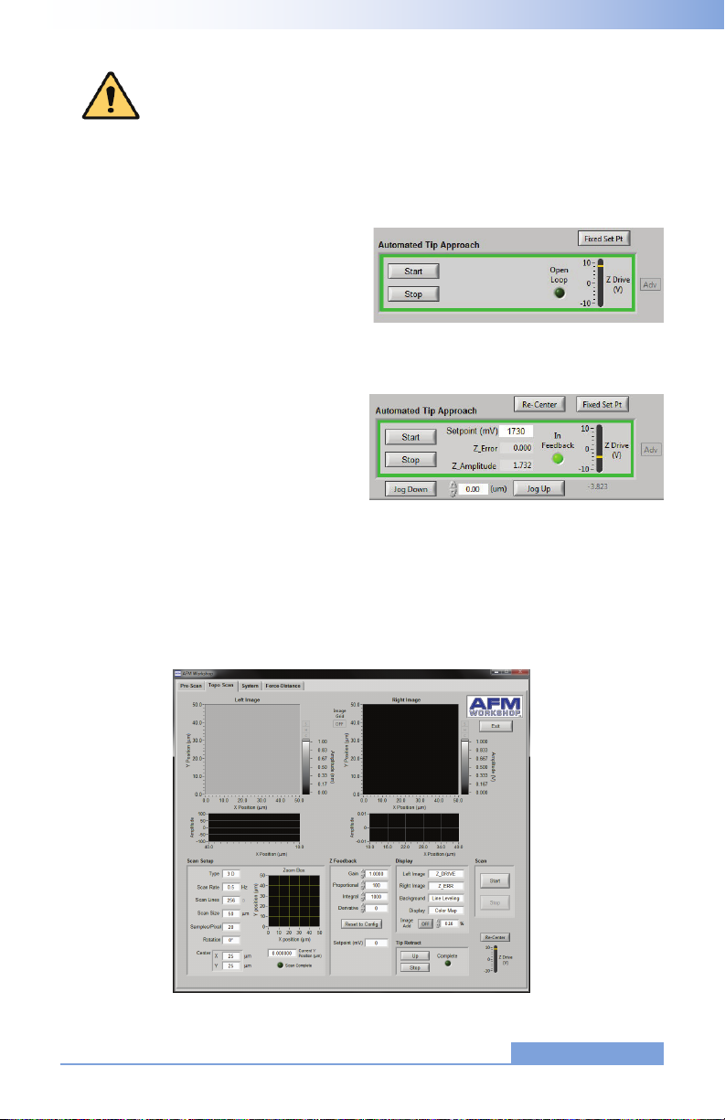
A small Adv button on the far right of the Z
Drive range allows advanced users to manu-
ally manipulate tip approach, by altering the
setpoint and jogging the Z motor. This can
achieve a lighter feedback for high resolution
scanning. See section 6 for more information
on high resolution scanning.
3.2.1.7 Automated Tip Approach
The Automated Tip Approach button starts
the process of the probe moving toward
the surface. A woodpecker motion is used,
which results in noticeable clicking sounds
from the microscope stage. This sound is
from two sources: the stepper motor being
energized and the Z piezoelectric ceramic
being retracted. When the system is
engaged in feedback, the Open Loop button
will light up and say “In Feedback.”
CAUTION: Before activating the Range Check function, make sure that the
probe is moved away from the sample surface. If the probe is too close to
the surface, the probe may be damaged.

Section 3-6 V 1.1 / LS-AFM Users Guide
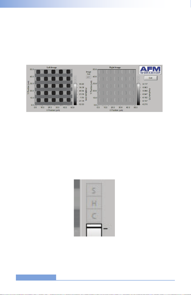
3.2.2.1 Image Window
Two images are displayed simultaneously while scanning. The type of images and their
appearances are selected in the Display menu window. As the images are displayed, there
is a constant normalization of the data so that the images appear in full scale.
SHC buttons on the right side of the Image Windows allow users to open the scans in
a larger window and adjust the color scheme and histogram in real time. Each of the win-
dows is opened by clicking on S, H, or C; the window can be closed by re-clicking on the
S, H, or C.

V 1.1 / LS-AFM Users Guide Section 3-7
3.2.2.2 Oscilloscope Window
A Z vs. X position plot of the probe as it scans across a surface is plotted in two screens. The
data plotted is selected in the Display window.
The histogram (H) can be adjusted
by moving the red and green verti-
cal bars.
The C button allows the user to
choose between a number of color
schemes.
The S button opens a larger ver-
sion of the image in a new window.

Section 3-8 V 1.1 / LS-AFM Users Guide
3.2.2.3 Scan Setup
All of the parameters required for scanning are presented in the Scan Setup window. Once
scanning is started, these parameters may not be changed. The parameters are:
1. Type: The scan can be either 2-D, which scans just the x-axis, or 3-D, which scans both
the x- and y-axis.
2. Scan Rate: The rate in Hertz that the
probe is scanned across the surface
(max 2 Hz).
3. Scan Lines: The number of lines in the
y-axis and the number of pixels mea-
sured in the x-axis.
4. Scan Size: The range of the scan,
from 0.1 micron to either 15 or 50
microns (depending on scanner size).
5. Samples/Pixel: The number of data
points signal averaged per pixel while
a scan is being taken.
6. Rotation: A scan can be completed
with 0° or 90° rotation.
7. Center: The center of the scan in x and y coordinates.
8. Current Y/X Position: The position of the probe along the y-axis as a scan is taken at
0°, along the x-axis for a 90° scan.
9. Scan Complete: This indicator turns green when a scan is completed.
10. Zoom Box: This shows the position and size of the scan in a grid. The scan area must
be within the zoom box area.
3.2.2.4 Z Feedback
All of the parameters for maintaining feedback are provided
here. The parameters are:
1. Gain: Scale factor for the feedback control signal.
2. Proportional: Scale factor for the proportional term in the
PID feedback controller.
3. Integral: Scale factor for the integral term in the PID
feedback controller.

V 1.1 / LS-AFM Users Guide Section 3-9
Source of signals displayed in the “Display Left/Right” drop down boxes
Light Lever
Photo-Detector
Phase/Amplitude
Demodulator
Comparator GPID H.V. Amp Z Piezo
Strain Gauge
Setpoint
Z SENSE
Z AMP Z PHASE
T-B L-R T+B
Non-Vibrating
Signal
Vibrating
Signal
Z ERR Z DRIVE
3.2.2.5 Display
There are several options for changing the appearance
of the images displayed in the Scan window. They are:
1. Left Image: The source of the image displayed in
the left image window.
2. Right Image: The source of the image displayed
in the right image window.
3. Background: When Line Leveling is selected, the
background is subtracted from the image one line
at a time.
4. Display: Two types of displays may be selected:
Color Map and Light Shaded.
5. Image Add: This function allows the user to over-
lay the left and right images while scanning. The
opacity may be adjusted by the % value.
CAUTION: If the Z Feedback parameters are too high, the Z ceramic can
begin to oscillate and potentially cause damage to the ceramic.
4. Derivative: Scale factor for the derivative term in the PID feedback controller.
5. Setpoint: Parameter that controls the magnitude of interaction between the probe and
surface.

Section 3-10 V 1.1 / LS-AFM Users Guide
3.2.2.6 Tip Retract
After scanning a sample, this function is used to move
the tip away from the surface. The Tip Retract function
should always be used to assure that the probe does not
get damaged after scanning.
3.2.2.7 Scan
These buttons allow the user to start and stop scans.
3.2.3 System Window
The system tab has several parameters that control the functionality of the TT-2 AFM. These
parameters should not be changed without a detailed understanding of the function that is
being modied. Incorrect use of the system functions can damage the TT-2 AFM.
System tab in non-vibrating mode
System tab in vibrating mode

V 1.1 / LS-AFM Users Guide Section 3-11
NOTE: A new high voltage gain value is entered into the system when tip
approach is being undertaken. Without enabling tip approach, the Z setting
will not change.
NOTE: Changing the calibration values
will change the scale on images mea-
sured with the TT-2 AFM. Only change
the values when calibrating with a refer-
ence sample.
NOTE: The Save button will turn green
when pushed. However, the new values
will not be saved in the Scanner congu-
ration le until the Exit button is pushed
in the Topo Scan window. The user must
have administrator rights in order to save
the calibration values.
3.2.3.3 XYZ Calibration
The calibration values in this sub-window can be adjusted when scanning a standard refer-
ence sample. Appendix C explains how to calibrate the TT-2 AFM in detail.
3.2.3.1 Tip Approach
This sub-window controls the step used for the stepper motor in tip approach. These func-
tions are very useful for high resolution imaging (see section 6). The Tip Approach motor jog
value automatically adjusts to changes in the Z HV Gain (reduces by a factor of 1/3). When
the advanced tip approach options are not selected on the Pre-Scan tab, the Tip Approach
motor jog function moves to the Other Controls sub-window.
3.2.3.2 Z Parameters
The high-voltage amplier that drives the Z ceramic in the
XYZ scanner has 15 gain settings. This function allows reduc-
tion of the Z gain of the high-voltage amplier. Reducing the
gain reduces the dynamic range of the ceramic, which also
reduces the noise oor of the instrument.
Vibrating mode values Non-Vibrating mode values

Section 3-12 V 1.1 / LS-AFM Users Guide
3.2.3.4 XY Parameters
Adjusting these parameters will alter the voltages applied to
the X and Y ceramics, which can be used for measuring and
reducing Z noise in images (see Appendix D for instructions
on how to complete a Noise Floor). XY HV Gain allows gain
reduction of the X and Y high-voltage ampliers, similar to Z
HV Gain. Reducing the X and Y GPID settings will decrease
strain gauge activity. This will affect linearization, but will also
reduce the noise oor of the system.
3.2.3.5 Other Controls
1. Beeper: Enables a beeper that noties an operator that a scan is completed with an
audible tone. (Speakers must be enabled)
2. Amplitude Value: Displays the current Z amplitude used in Tip Approach. This value
should correspond with the Selected Frequency on the Pre Scan tab.
3. Feedback Limit: This function controls the feedback LED that turns green when Tip
Approach has achieved feedback. If the feedback light is ickering when the tip is in
feedback, increase this value by 0.01V.
4. Extend Factor: This function determines the percent decrease of vibrational amplitude
of the probe in vibrating mode. The typical range for extend factor is 0.7-0.95, with 0.95
creating a 5% reduction in vibrational amplitude for high resolution scanning.
5. Extend Delta: This function determines the amount of probe deection on the surface
in non-vibrating mode. Extend delta is typically 0.1, meaning the Top-Bottom signal will
deect by 0.1V before feedback is initiated.
6. Tip Approach motor jog: This function will appear in the Other Controls sub-window
when the advanced tip approach options are not visible.
Other Controls for vibrating mode Other Controls for non-vibrating mode

V 1.1 / LS-AFM Users Guide Section 3-13
3.2.4 Force/Distance Curves
Force/distance curves are created by measuring the deection of the cantilever as the sam-
ple is moved towards and then away from the probe at the end of the cantilever. The shape
of a F/D curve depends primarily on the cantilever stiffness and the thickness of a surface
contamination layer. For information about how to analyze F/D curves, see Appendix I.
Measurement of F/D curves is found on the Force-Distance tab.
1. Down: The distance in nanometers that
the sample will be moved away from
the probe when the F/D curve measure-
ment is initiated.
2. Up: The distance in nanometers that
the sample will be moved up from the
feedback position during the F/D curve.
During this part of the curve, the probe
is touching the sample surface.
3. Rate: The rate or velocity of the sample
as it is moved towards and away from
the probe.
The AFM must be in feedback in non-vibrating mode before a F/D curve is measured. There
are three important parameters that must be set before the F/D curve is measured. They are: