PicoQuant GmbH HydraHarp 400 Software V. .0.0.1
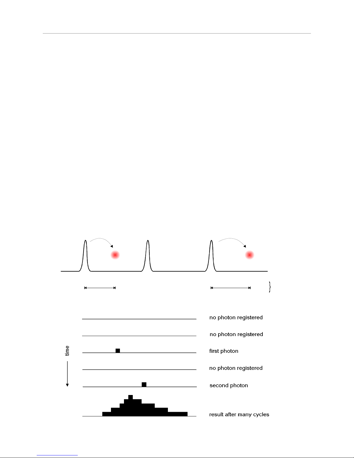
The histogram is collected in a block of memory, where one memory cell holds the photon counts for one
corresponding time bin. These time bins are often (historically) referred to as time channels. In practice, the
registration of one photon involves the following steps: first, the time difference between the photon event and
the corresponding excitation pulse must be measured. For this purpose both signals are converted to electrical
signals. For the fluorescence photon this is done via the single photon detector mentioned before. For the
excitation pulse it may be done via another detector if there is no electrical sync signal supplied by the laser.
Obviously, all conversion to electrical pulses must preserve the precise timing of the signals as accurately as
possible. The actual time difference measurement is done by means of fast electronics which provide a digital
timing result. This digital timing result is then used to address the histogram memory so that each possible
timing value corresponds to one memory cell or histogram channel. Finally the addressed histogram cell is
incremented. All steps are carried out by fast electronics so that the processing time required for each photon
event is as short as possible. When sufficient counts have been collected, the histogram memory can be read
out. The histogram data can then be used for display and e.g. fluorescence lifetime calculation. In the following
we will expand on the various steps involved in the method and associated issues of importance.
2.1. Count Rates and ingle Photon tatistics
It was already mentioned that it is necessary to maintain a low probability of registering more than one photon
per cycle. This was to guarantee that the histogram of photon arrivals represents the time decay one would
have obtained from a single shot time–resolved analog recording (The latter contains the information we are
looking for). The reason for this is briefly the following: Due to dead times of detector and electronics for at
least some tens of nanoseconds after a photon event, TCSPC systems are usually designed to register only
one photon per excitation / emission cycle. If now the number of photons occurring in one excitation cycle were
typically >1, the system would very often register the first photon but miss the following one or more. This
would lead to an over–representation of early photons in the histogram, an effect called ‘pile–up’. This leads to
distortions of the fluorescence decay, typically the fluorescence lifetime appearing shorter. It is therefore crucial
to keep the probability of cycles with more than one photon low.
To quantify this demand, one has to set acceptable error limits and apply some mathematical statistics. For
practical purposes one may use the following rule of thumb: In order to maintain single photon statistics, on
average only one in 20 to 100 excitation pulses should generate a count at the detector. In other words: the
average count rate at the detector should be at most 1 % to 5 % of the excitation rate. E.g. with the diode laser
PDL 800–B, pulsed at 80 MHz repetition rate, the average detector count rate should not exceed 4 Mcps. This
leads to another issue: the count rate the system (of both detector and electronics) can handle. Indeed 4 Mcps
may already be stretching the limits of some detectors and usually are beyond the capabilities of older TCSPC
systems. Nevertheless, one wants high count rates, in order to acquire fluorescence decay histograms quickly.
This may be of particular importance where dynamic lifetime changes or fast molecule transitions are to be
studied or where large numbers of lifetime samples must be collected (e.g. in 2D scanning configurations). This
is why high laser rates (such as 40 or 80 MHz from the PDL 800–B) are important. PMTs can safely handle
TCSPC count rates of up to 10 Mcps, standard (passively quenched) SPADs saturate at a few hundred kcps,
actively quenched SPADs may operate up to 5 Mcps but some types suffer resolution degradation when
operated too fast. Old NIM based TCSPC electronics can handle a maximum of 50 to 500 kcps, newer
integrated TCSPC boards may reach peak rates of 5 to 10 Mcps. With the HydraHarp 400, in each channel
average count rates of 6 Mcps and peak rates up to 12.5 Mcps can be collected. It is worth noting that the
photon arrival times are typically random so that there can be bursts of high count rate and periods of low count
rates. Bursts of photons may still exceed the average rate. This should be kept in mind when comparing count
rates considered here and elsewhere. The specifications for TCSPC systems may interpret their maximum
count rates differently in this respect. This is why another parameter, the so called dead–time is also of interest.
This quantity describes the time the system cannot register photons while it is processing a previous photon
event. The term is applicable both to detectors and electronics. Dead–time or insufficient throughput of the
electronics do not usually have a detrimental effect on the decay histogram or, more precisely, the lifetime to be
extracted from the latter, as long as single photon statistics are maintained. However, the photon losses
prolong the acquisition time or deteriorate the signal to noise ratio (SNR) if the acquisition time remains fixed. In
applications where the photon burst density must be evaluated (e.g. for molecule transition detection) dead–
times can be a problem. The HydraHarp 400 has an extremely short dead time of typically less than 80 ns,
imposing the smallest losses possible with instruments of comparable resolution today.
Page 7