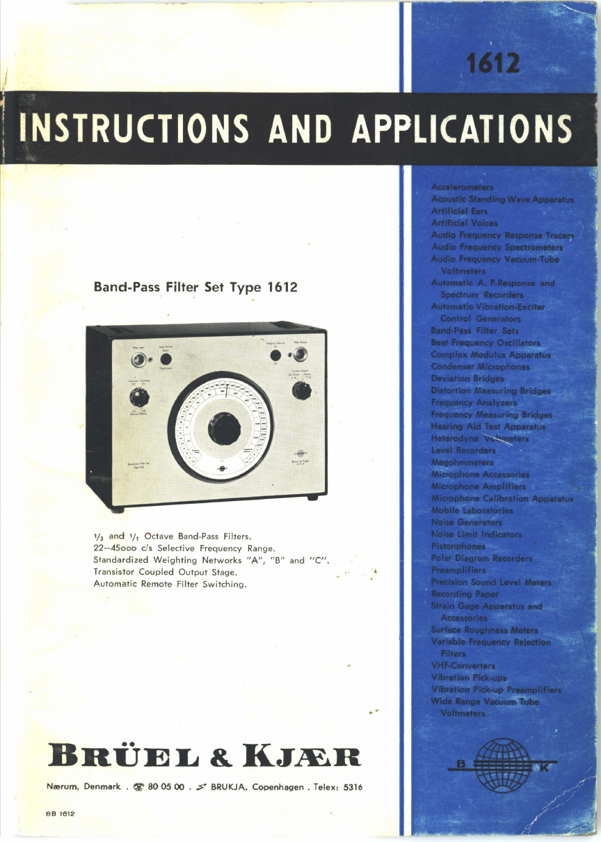
Bruel & kjaer 1612 User guide

Band-Pass. Filte_r Set Type 1612

·•

~

i

.

113

and

1/

1

Octave

Band-Pass Filters.

22

-

45ooo

c/s Selective Frequency Range.

Standardized

Weighting

Networks

"A",

"B"

and

"C".

Transistor

Coupled

Output

Stage.

'4

Automatic

Remote Filter

Switching.

_.,

BHUEL&KJ&H

Ncerum, Denmark. .

~

80

05 00

.

~

BRUKJA,

Copenhagen

. Telex: 5316

BB

1612

Band-Pass

Fi

Iter

Set

Type 1612

Reprint

june

1965

Contents

Introduction .................................................. 5

Description ................................................... 8

Control Knobs and Terminals ............................. 24

Operation .................................................... 26

Accessories and Combined Units ....................... 49

Applications .. ..

.....

...... ......·.

..

.. .. ..

.....

............... 54

Specification ... ... ..

....................

.. ...

..

..........

.

....

73

0.

Introduction

Filters Handling

Noise

with

Uniform

Spectrum Density.

In

investigations

where

narrow

bands

are

to

be

selected

from

noise

with

uniform

spectrum

density

(white

noi

s

e)

the

use

of

band-pass

f~lters

is

necessary.

Ideally

such

filters

should

display

zero

attenuation

within

the

pass-band

and

infinite

attenuation

elsewhere,

i.e.

filters

which

provide

rectangular

amplitude

vs.

frequency

characteristics.

Refer

also

Fig. 0.1.

Such

filters

cannot

be

produced

in

practice

by

passive

components

but

they

should

display

characteristics

as

near

as

possible

to

that

of

the

ideal

filters,

i.e.

a

flat

pass-band

and

steps

skirts.

Effective

Bandwidth

of

a

practical

filter

is

equal

to

the

bandwidth

of

an

ideal

filter

which

has

uniform

transmission

in

its

pass-band

equal

to

the

maximum

transmission

of

the

specified

filter

and

transmits

the

same

power

of

white

noise

as

the

specified

filter.

The

effective

bandwidth

of

a

specified

filter

can

be

determined

by

firstly

plotting

the

amplitude

vs.

frequency

response

of

the

filter

in

a

graph

with

a

linear

ordinate

showing

the

ratio,

transmission

at

the

particular

frequencies

to

the

maximum

transmission,

and

with

an

abscissa

showing

the

relative

f

frequency

f;

,

where

fo

equals

the

center

frequency

of

the

filter.

Refer

also

Fig. 0.1.

Secondly,

the

ordinates

of

this

characteristic

are

now

squared

and

plotted

in

the

same

co-ordinates

as

above.

Thirdly,

the

area

so

enclosed

by

the

new

characteristic

and

the

zero

line

(hatched

in

Fig. 0.1)

divided

by

maximum

height

of

same

area

gives

the

effective

bandwidth

of

the

specified

filter.

In

many

noise

measurements

it

is

convenient

to

know

the

correction

factor

in

dB

for

the

individual

filters

which

have

to

be

applied

to

the

measured

quantities

due

to

the

fact

that

the

practical

filters

do

not

have

a

....

!laracteristic

identical

to

the

ideal

filter.

This

correction

factor

can

be

derived

from

the

effective

bandwidth

of

the

individual

filters

as

this

is a

measure

for

the

noise

power

the

filter

allows

to

pass.

.

Effective

Bandwidth

Correction

Factor

(dB) = 10 X

log

B d

'd

h f

ld

1

F'l

an

w1

t o

ea

1

ter

When

relative

noise

measurements

are

made,

it

is

also

of

great

convenience

to

know

how

much

this

correction

factor

deviates

from

filter

to

filter.

The

5

·

u;

-~

.

0.4

c:

_g

0.

3i-

-i--t----H'-

~

] 0.

2+-

-f----1--1+-

&

--Frequency

Fig. 0.1. Characteristics

of

an ideal

and

practical filter. Note

both

co-ordinates

are linear.

deviation

in

the

factor

could,

additionally,

be

referred

to

a

filter

in

the

middle

of

the

range,

for

example

at

1ooo

Hz

(c/s).

If

the

deviation

of

the

correction

factor

would

be

zero

(which,

of

course,

will

be

impossible

for

practical

filters)

and

the

filters

in

the

range

considered

display

constant

relative

bandwidth,

the

output

noise

level

from

the

filters

would

increase

by

exactly

10

dB

/

decade~

3 dB/

octave

as

the

r.m.s. voltage

white

noise

is

proportional

to

the

square-root

of

its

effective

bandwidth.

The

deviation

in

the

correction

factor

of

the

individual

filters

will

thus

.:.:

qual

the

deviation,

which

can

be

expected

from

this

3 dB/

octave

line.

Octave.

When

dealing

with

acoustics,

an

octave

is

an

expression

of

a

relative

measure

of

frequency,

i.e. 1 ootave

above

or

below

a

certain

frequency

f•

means

2 X

fo

or

1h

X

fo

respectively.

:Mathematically

it

is

expressed

by:

__!_=

2D

fo

where

n

may

be

positive,

negative,

a

fraction

or

a

number

of

octaves

and

f•

~he

frequency

to

which

the

frequency

f is

referred.

6

By

taking

the

logarithm

on

both

sides

of

the

equation

above,

it

is derived:

f

log10 -= n X o.3010

fo

from

which

f

or

n

for

a given n

or

f

respectively

can

be

calculated.

In

Fig. 0.2 will

be

found

a

graph

where

n, positive

and

negative, is

plotted

f

versus

relative

frequency

fo

Example:

+

~

octave = + o.5 octave

6

•6

reads

_!_

=

1.41

fo

.5

_!_

octave = - o.17 octave 6

6

reads

_!_

l'

o = 0.

89

+ 4

6

·i

~

+

~

8

t.

~

05

~_1_

fa 0.6 0.7 0.8 0.9 /

1

I-'

~

1t;

.2

~:l

.3 v

~

0:

l:

/ 6

.4 v t

.5 v

6 /

[,_

7 / 6

8 I/ t

]/

9

1[/

-

/

11

1/

v

l/

/v

/

v

12

1.3

1.4

1.5

1.6

1.7

Fig. 0.2. Graph for

octave

into

relative

p-1

1/

v 0.9

0

0.7

0

.6

0.5

0.4

.d

0

2t

.1 I

1.8 1.9

20

__,...L

fa

convert

ing

ncy

,

freque

and

Pice versa.

7

Description

General

9

Input

Circuit

. . . . . . . . . . . . . . . . . . . . . . . . . . . . . . . . . . . . . . . . . . . . . . . . . . . . . .

10

Filters

. . . . . . . . . . . . . . . . . . . . . . . . . . . . . . . . . . . . . . . . . . . . . . . . . . . . . . . . . . . . .

10

1

h

Octave

Filters

. . . . . . . . . . . . . . . . . . . . . . . . . . . . . . . . . . . . . . . . . . . . . . . .

11

l!J.

Octave

Filters

.......................

.

......................

. . 16

Weighting

Networks

.

.........................

.

...........

...

........

18

"A",

"B"

and

"C"

.......................................

.

.....

.

..

18

Low

Frequency

Cut-off

. . .

...

. . .

.....................

.

...........

19

Selection

of

Filters

and

Weighting

Networks

. . . . . . . . . . . . . . . . . . . . . . . . . . 20

Remote

Control

. . . . . . . . . . . . . . . . . . . . . . . . . . . . . . . . . . . . . . . . . . . . . . . . . . 20

Extension

Filters

. . . . . . . . . . . . . . . . . . . . . . . . . . . . . . . . . . . . . . . . . . . . . . . . 20

Output

Stage

. . . . . . . . . . . . . . . . . . . . . . . . . . . . . . . . . . . . . . . . . . . . . . . . . . . . . . . .

21

Ove~all

Performance

of

Band-Pass

Filter

Set

. . . . . . . . . . . . . . . . . . . . . . . . . . 22

Trans1nission

. . . . . . . . . . . . . . . . . . . . . . . . . . . . . . . . . . . . . . . . . . . . . . . . . . . .

22

Non-linear

Distortion

....................................

.

.......

22

Signal-to-Noise

Ratio

...

.

...

.

...........

. . . .

..

.

..............

.

...

22

8

1.

Description

General.

The

Band-Pass

Filter

Set

Type

1612 is

intended

for

analysis,

selective

measurements

and

selection

of

noise

signals

in

1/3

or

1/1

octave

bands

covering

the

frequency

range

22-45ooo

Hz (c/s).

The

Filter

Set

contains

additionally

four

frequency

weighting

networks.

The

three

of

them

are

the

"A"

"B"

and

"C"

networks

the

characteristics

of

which

are

in

accordance

with

those

proposed

by

I.E.C.

for

Precision

Sound

Level

Meters.

The

fourth

network

gives a

linear

frequency

response

20-45ooo

Hz (c/s).

The

filters

and

weighting

networks

can

be

selected

successively

by

a 50

position

selector,

which

is

manual

as

well

as

remotely

operable.

An

input

transformer

and

an

output

transistor

stage

ensure

proper

matching

to

a

wide

range

of

source

and

load

impedances

respectively.

The

frequency

range

of

analysis

can

be

extended

to

cover

11-45ooo

Hz (c/s)

when

the

Filter

Set

is

combined

with

the

Extension

Filter

Set

Type

1620.

Fig. 1.1.

Block

diagram

of

Band-Pass Filter Set.

9

The

Band-Pass

Filter

Set

is

designed

to

be

combined

with

other

B & K

instruments,

for

example

the

Frequency

Analyzer

Type

2107,

the

Microphone

Amplifier

Type

2603

or

Type

2604

and

the

Precision

Sound

Level

Meter

Type

2203.

When

combined

with

the

two

first

of

the

four

mentioned,

an

instrumentation

is

obtained

which

has

data

identical

to

the

B & K A.F.

Spectrometer

Type

2112.

In

measurements

where

random

noise

is

required

as

test

signal

the

Filter

Set

can

be

combined

with

the

B & K

Random

Noise

Generator

Type

1402.

Noise

bands

of

1/3

or

1/1

octave

widths

can

be

supplied

from

such

a

combination.

When

employing

the

Filter

Set

together

with

the

above

mentioned

instruments,

except

the

Precision

Sound

Level

Meter,

the

supply

for

the

transistor

output

stage

is

derived

from

the

associated

instrument

via

the

Filter

Set

input

terminal.

Block Diagram.

The

basic

design

of

the

Band-Pass

Filter

Set

is

illustrated

in

Fig.

1.1.

The

input

circuit

(to

the

left

in

the

figure)

allows

the

input

signal

to

be

applied

either

directly

to

the

filter

or

via

an

input

transformer.

The

filters

and

weighting

networks,

the

inputs

of

which

are

paralleled,

are

selected

at

the

outputs

by

the

filter

switch.

From

this

switch

the

signal

passes

the

transistor

stage

to

the

output

of

the

Filter

Set.

The

remote

filter

selection

is

provided

by

a

built-in

electro-mechanic

device,

which

can

be

controlled

by

an

external

contact

in

series

with

a d.c.

supply.

Input Circuit.

A

selector

and

an

input

transformer

constitutes

the

input

circuit.

The

selector

INPUT

SWITCH

has

two

positions.

In

the

one

position

the

signal

is

applied

direct

to

the

input

of

the

filters

and

weighting

networks.

In

the

other

position

a

step

down

transformer

10 : 1 is

coupled

in

series

with

the

filter

and

weighting

network

inputs.

Inserting

the

transformer

allows

a

higher

source

impedance

up

to

1ooo

n

to

be

used

in

conjunction

with

the

filters

in

relation

to

the

10 n

required

when

the

signal

is

applied

direct.

The

10

time

·s

(20

dB)

lower

sensitivity

occuring

when

the

transformer

is

switched

in,

must

be

taken

into

consideration

during

measurements.

To

keep

the

magnetic

flux

in

the

filter

cores

below

the

value

of

saturation

the

voltage

on

the

filter

inputs

should

not

be

higher

than

1.4

volts

peak.

Consequently

by

inserting

the

transformer

the

peak

voltage

on

the

"Filter

Input"

terminal

can

be

14

volts.

Filters.

By a

switch

FUNCTION

SELECTOR

it

is

possible

to

select

sets

of

filters,

either

'Qlith a

bandwidth

of

1

/a

octave,

or

with

a

bandwidth

of

lA.

octave.

The

cente~

ucyuencies

of

both

types

of

filters

are

placed

in

accordance

to

the

ISO

standards

for

acoustic

measurements.

tO

1

/a

Octave Filters.

Design.

The

Filter

Set

is

equipped

with

33

filters

having

center

frequencies

as

given

in

the

table

below

from

which

also

the

filter

bandwidth

in

cycles

per

second

can

be

found.

Center

Frequency

I

Bandwidth

at

3 dB

Center

Frequency

I

Bandwidth

at

3 dB

Hz

(c/s) Hz (c/s)

Hz

(c/s) I

Hz

(c/s)

Approx.

25 5.8 1000 230

31.5 7.3 1250 290

40 9.2 1600 370

50 11.6 2000 460

63 14.5 2500 580

80 18.3 3150 730

100 23 4000 920

125 29 5000 1160

160 37 6300 1450

200 46 8000 1830

250 58 10000 2300

315

73

12500 2900

400 92 16000 3700

500 116 20000 4600

630 145 25000 5800

800 183 31500 7300

40000 9200

A

single

filter

consists

of

three

resonant

circuits

coupled

together

as

shown

in

Fig.

1.2.

The

first

two

circuits

will

give

rise

to

a

two-topped

frequency

response,

as

shown

in

Fig.

1.3 left.

The

third

gives a

single

top

which

raises

the

valley

between

the

two

tops,

so

that

a

resultant

curve

having

a

relatively

flat

band-pass

and

steep

sides

as

shown

in

Fig.

1.3

right

is

obtained.

Because

Hum compensation coils

460219

Fig. 1.2. Schematic diagram

of

a single 1/9 octave filter unit.

11

Attenuation

db

fo

m

I•

n

Frequency

+60220

Fig. 1.3.

Frequency

characteristics illustrating

the

function

of

a 1/3 octave

filter unit.

the

two

tops

do

not

have

the

same

height.

The

third

resonant

frequency

must

be

placed

unsymmetrically

to

obtain

the

desired

band-pass,

and

the

resultant

response

curve

will

have

two

humps,

a

broad

one

and

a

narrow

one.

The

input

impedance

response

of

the

paralleled

filters,

will

be

a

wave-shaped

curve,

varying

between

approximately

500

ohms

and

2ooo

ohms,

so

that

the

impedance

is

high

at

the

center

frequencies

and

low

at

the

band

limits

(see

also

Fig.

1.4).

kSl

~

2

c

!

1,5

.~

l

1

0,5

0 2 5

10

100

kQ

~

75

c

al

.

~

50

~

25

0

--

Frequency

A

2

10

100

-Frequency

2 5 2 5 2 5

1000 10000 100000 C/S

162487

A

II

I'

v -

1000 10000 100000 C/S

(62-+88

Fig. 1.4.

Typical

input

impedance

of

Band-Pass Filter

Set

measured

or.

FILTER

INPUT.

Extension

Filter Set

Type

1620 has been connected. FUNC-

TION

SELECTOR

on "1/3 Octave, 0

dB"

and WEIGHTING

NETWORK

"On"

.

(a)

INPUT

SWITCH

on "Direct"

(b)

INPUT

SWITCH

on

"Transformer"

12

The

input

voltage

will

therefore

also

vary

up

and

down

if

the

output

impedance

of

the

input

amplifier

it

not

made

low.

At a

source

impedance

of

approximately

10

ohms

the

voltage

across

the

filters

will

only

vary

approximately

1.5

%.

To

keep

the

transients

in

the

filters

to

a

minimum

all

the

filter

inputs

are

coupled

in

parallel.

Furthermore,

the

filters

are

pre-loaded,

and

the

change

in

load-when

the

Filter

Switch

connects

the

output

amplifier

to

the

different

filters-is

thus

negligible.

Frequency Response.

The

frequency

response

of

a

filter

is

flat

to

within

± 1

h dB

over

approximately

1

,4

octave.

At

the

band

limits,

i.e. lk

octave

from

the

center

frequency,

the

attenuation

is

approximately

3 dB. See Fig. 1.5.

However,

due

to

the

rather

steep

slope

of

the

filter

curves

at

these

points,

the

frequency

characteristics

of

two

neighbouring

filters

cannot

be

expected

to

intersect

exactly

at

the

3 dB

point.

This

is

easy

to

understand,

because

1/3

octave

25 •

31.5

C/5

and

80

C/5

to

40

k c/5

-2

-1

/3

-11j3

-1

-2J3

-1J3

0.25

0.5

60

25.31.5c/5 and 80

C/5

to

40k

C/5

0

+1/3

+2/3

+1

+11J3

+12/3

+2 octave

1 2 4

_!_

Frequency__..

fo

16191~

1000

C/5

and

1600C/S

Fig. 1.5. Detailed 1/9 octave filter characteristic derived

from

sine-wave

signals.

13

ooooooooooooooo

ooo

ooooooo

oooooooooo

oooooooo

15

db

5

:g

c

~

1

10

100

10000

20000

c/

•

40000

A I C

U...

1000

10000

c/s

(~&n

t21TJ)

,.,

• c

LJn.

·

Frequency~

!6/910

Fig. 1.6.

Complete

set

of

filter

charackristics

when

Filter

Set

is

in

1/3 octave

conditim<.

a

displacing

of

the

center

frequencies

of

the

two

filters

by

only

1 %

in

opposite

directions,

will

cause

the

intersection

to

take

place

at

a

point

1.7 dB

higher

or

lower

than

the

3

dB

point.

If

the

width

of

one

filter

curve

is

changed

by

1

%,

the

point

of

intersection

is

changed

by

o.2 dB.

The

attenuation

approximately

at

± lh

octave

from

the

center

frequency

is

20

dB,

and

at

± 1

octave

52 dB.

It

has

been

impossible

to

obtain

sufficiently

high

quality

factors

for

the

coils

at

some

frequencies

below

80

c/s

without

lowering

the

stability

or

making

the

filters

larger

and

heavier.

The

filter

curves

will

therefore

not

be

of

the

same

quality

at

these

frequencies,

as

there

will

be

only

top,

and

the

"flat"

part

is

about

lk

octave

wide.

The

attenuation

of

these

filters

is

up

to

4 dB

at

the

band

limits,

from

14

to

20 dB

at

± 1

h

octave,

and

from

42

to

50 dB

at

1

octave

away

from

the

center

frequency.

Effective

Bandwidth.

The

effective

bandwidth*)

of

the

%

octave

filters

is

9 %

greater

than

the

bandwidth

of

an

ideal

lh

octave

filter

which

trans-

mission

in

the

pass

band

is

equal

to

that

of

the

Filter

Set

when

in

con-

dition

"Lin."

(20-45ooo

Hz (c/s)).

Due

to

tolerances

in

the

filter

production,

the

mentioned

correction

of

+ 9 %

to

the

bandwidth

may

be

found

to

lie

between

0 %

and

+20

%.

In

some

measurements

it

may

be

necessary

to

make

a

correction

to

the

measured

values

because

of

the

9%

greater

bandwidth.

The

correction

factor

*)

in

dB

then

equals

-o.4

dB.

The

deviation

of

this

factor

will,

due

*)

Vide also

Introduction,

para

Filters

Handling

Noise

with

Uniform

Spectrum

Density.

14

to

the

production

tolerances

be

:::!::

o.4 dB,

which

means

that

the

greatest

relative

deviation

will

be

within

these

limits.

Phase

Response.

Due

to

the

nature

of

the

filters

they

will

cause

a

pltase

distortion,

which

is

shown

in

Fig.

1.7,

together

with

the

amplitude

response

of

the

filter

top.

The

hatched

area

indicates

the

limits

within

which

the

different

filter

curves

for

one

apparatus

are

expected

to

lie.

1!3

Octave

Filter

db

c:

0

] 10

<

15

20

270°

180°

goo

lo~

c:

oo

0

~

goo

:0

...

Ill

c

.J::. 180°

Q_

Frequency -

16

36-'lf

/:<'ig.

1.7. Phase response

of

Filter set in 1/3 octave condition,

shown

together

with

the

respective

amplitude

characteristics.

Hum

Compensation.

To

reduce

the

induction

of

hum,

in

some

of

the

low

-

frequency

filters,

occuring

from

magnetic

fields

created

by

nearby

mains,

transformers,

or

electrical

machinery,

the

filters

are

provided

with

hum

compensation

coils

as

seen

in

Fig.

1.2.

By

this

means

a

very

low

hum

level

is

obtained.

16

1/t Octave Filters.

Design.

The

11

octave

filters

are

obtained

by

internally

combining

the

%

octave

filters

in

units

of

three

in

such

a

manner

that

the

bandpass

of

the

individual

units

will

cover

a

complete

octave.

The

center

frequencies

of

the

'

octave

filters

are

given

in

the

table

together

with

the

filter

bandwidth.

Center

Frequeney

Hz (e/s)

31.5

63

125

250

500

1000

Maximum

steep-

ness

about

100dbfoctave

-2

-11j2 -1

0.5

0.25

I

Bandwidth

at

3 dB

Center

Frequeney

I

Bandwidth

at

3 dB

-1j2

Hz (e/s)

Approx.

22

45

89

177

353

707

db

c

.2

.....

0

:::J

c

~

j

0

1

20

30

liJ

50

60

Hz (e/s) Hz (e/s)

Approx.

2000

1410

4000

2810

8000

5600

16000 11200

31500

I

22300

16000

C/S

-

Lt."'si-~---

-/:4-~

-

['i

~--

-,\\

r,

r . \

hI 1

000

qs

I

125

C/S

f +3db

I

1 octave

125cfs to 31.5kcf

+Y2

+1

+11f2

2

Frequency---...

+2

octave

4 f -

"fa"

161913

+2

Odb

Fig.

1.8.

Detailed 1/1 octave filter characteristics derived from sine-wave

signals.

16

-

O

DDDO

OOO

D

DDODD

DDD

DO

OOOO

OO

O O

OOOO

DD

ODDDOO

O D

15

db

.5

b

;:,

c

I 10000 20000 cl•

<1

0000

~

I C

1.11\.

1 O

10

100

1000

10000

c/s

'~'

"

'"

• ' c

""

Frequency-

f6f916

Fig.

1.9.

Complete set

of

filter characteristics

when

Filter Set

is

in 1/1 octave

condition.

db

10

c

0

]

<

20

30

630°

540°

360°

180°

lag

:5

oo

:;:;

~

lead

:0 180°

"'

0

.s:.

a.

360°

540°

630°

Octave

Filter

/.

....

---

.....

/(/

-"

'\

/A

~~;

.

5%

/rff

\',

/1V

~~\

fj

~\

f!

.

~

31.5 kC/s

~

I

v~J~s

.f

h'l

f

.I

~f

~

Fig. 1.10. Phase response

of

Filter

Set

in

111

octave condition,

shown

together

with

the

respective

amplitude

characteristics.

%

~

t-6 t-6

1fs

-o+

1!6

2/6

=¥s

"6

!j(;

octl:lve

Frequency

-r6f9J-9

17

Due

to

the

circuit

used

for

connecting

three

lh

octave

filters

to

a

lA

octave

filter

a

certain

voltage

drop

is

unavoidable.

This

voltage

drop

is

made

equal

to 10 dB,

which

should

be

taken

into

account

during

measurements.

The

FUNCTION

SELECTOR

switch

is

therefore

in

position

"Octave"

also

marked

"10

dB".

Frequency

Response.

The

filters

are

adjusted

so

that

the

deviations

in

the

pass

band

between

peaks

and

valleys

are

within

± 1 dB;

for

the

31.5 Hz (c/s)

and

63

Hz

(c/s)

within

± 2 dB. At

the

band

limits,

i.e. ± lh

octave

from

the

center

frequency,

the

attenuation

is

approximately

3 dB,

vide

Figs.

1.8

and

1.9.

The

attenuation

at

± 1

octave

is

approximately

35 dB,

being

somewhat

less

for

the

filters

at

the

lower

frequencies.

Phase

Response.

The

phase

response

curves

of

the

octave

filters

are

shown

in

Fig. 1.10,

together

with

the

amplitude

response

of

the

filter

top.

The

curves

for

the

different

filters

are

expected

to

lie

within

the

hatched

area.

Weighting

Networks.

"A",

"B"

and

"C".

The

three

networks

are

mainly

designed

as

illustrated

in

Fig. 1.11.

The

frequency

response,

each

sinusoidal

component

of

the

signal

is

given

in

Fig. 1.12.

In

the

table

below

will

be

found

the

respective

tolerances.

For

comparison

the

I.E.C.

tolerances

for

ordinary

Sound

Level

Meters

are

also

given.

IR

1636+0

Pig. 1.11.

Schematic

diagram

of

weighting

networks

for

sound

level

measurements.

BRUEL & KJAER 1612 User guide

Popular Water Filtration System manuals by other brands