Nicoya OpenSPEC Operation manual

NICOYA LIFESCIENCES
Operation and Service Manual V1.0
Last Updated: April 20, 2016 (V1.0)
[email protected]om
OpenSPEC

2
Table of Contents
Table of Contents ..................................................................................................................................................2
SAFETY AND PREPARATION FOR USE..................................................................................................................... 4
OPERATING CONDITIONS .................................................................................................................................................5
SPECIFICATIONS .............................................................................................................................................................6
CHAPTER 1: GETTING STARTED ........................................................................................................................ 7
1.1 INITIAL EQUIPMENT SETUP..................................................................................................................................7
1.1.1 Before any Steps are Taken......................................................................................................................7
1.1.2 Standard Equipment Supplies ..................................................................................................................7
1.1.3 Setting up the OpenSPEC™ Instrument....................................................................................................7
1.2 OVERVIEW OF OPENSPEC™ INSTRUMENT COMPONENTS.........................................................................................9
1.3 OPERATION GUIDELINES...................................................................................................................................10
1.3.1 Required Items .......................................................................................................................................10
1.3.2 Experimental Procedure.........................................................................................................................10
Taking New Reference Spectra......................................................................................................................................... 12
Loading a Sample ............................................................................................................................................................. 13
Optimizing Peak Tracking Manually ................................................................................................................................. 15
Recording events.............................................................................................................................................................. 17
1.3.3 Other Software Features........................................................................................................................18
Adjusting the Response Graph ......................................................................................................................................... 20
CHAPTER 2: TROUBLESHOOTING.................................................................................................................... 22
2.1 TROUBLESHOOTING .........................................................................................................................................22
CHAPTER 3: THEORY ...................................................................................................................................... 23
3.1 LOCALIZED SURFACE PLASMON RESONANCE.........................................................................................................23
3.2 REFERENCES...................................................................................................................................................24

3

4
Safety and Preparation for Use
Line Voltage
The OpenSPEC™operates from a 120/240 V, CSA Class 2 Approved power supply, with a frequency
between 50 and 60 Hz and 6 W power. Only use the power supply provided with your instrument.
Line Fuse
The line fuse is internal to the instrument and may not be serviced by the user.
Operate Only with Covers in Place
To avoid personal injury, do not remove the product covers or panels. Do not operate the product
without all covers and panels in place.
Serviceable Parts
The OpenSPEC™does not include any user serviceable parts inside. Refer service to Nicoya
Lifesciences Inc.
Additional Safety Notes
This unit has been thoroughly tested using standard biological buffer solutions such as Tris, PBS, and
Citrate buffer at neutral pH. Solutions at pH 2 to pH 12 have also been tested and can be used in the
system. Always evaluate the safety of the materials being used in the system before proceeding, and
utilize all appropriate and recommended safety precautions associated with the materials.
Do not stare into the LED as the bright light can damage the eye. Use appropriate safety eye
protection. Handle Sensor Chips inside of a fume hood with appropriate exhaust ventilation. Wear
personal protection equipment such as a laboratory coat, gloves, and safety glasses. In case of
insufficient ventilation, wear suitable respiratory equipment. Sensor Chips contain colloidal gold
particles which should not be inhaled, ingested, or contacted in any way.
This system is not water proof. Avoid actions which may result in liquid being spilled onto any part
of the system.
Always turn off the power to system when not in use.
It is recommended that the system be connected to a surge protected power Outlet.
Follow the recommended operating conditions below.

5
Operating Conditions
The following are the recommended operating conditions of the OpenSPEC™instrument and should
be followed for safety and performance purposes.
1. Read and follow all instructions provided.
2. For indoor use only.
3. For research use only.
4. Assure proper ventilation while in use.
5. Do not operate unattended and not designed for 24 hour continuous operation.
6. OpenSPEC™is not waterproof –do not spill liquids onto it and be very careful of leaks.
7. Do not operate the system in the presence of strong magnetic fields.
8. Dust may interfere with the instrumentation, it is recommended that compressed air be used
to remove any dust that may accumulate in the system after completing tests and that the
unit is stored with a closed lid.
9. It is the responsibility of the user to ensure the safety and appropriateness of the chemicals,
materials, and fluids being used in the OpenSPEC™.
10. Do not open the electronics compartment. Contact Nicoya Lifesciences Inc. if there is an
electrical problem and a customer service agent will assist you.
11. Turn off the OpenSPEC™immediately if a leak is detected.
This information is based on our present knowledge. However, this does not constitute a guarantee
for any specific product features and shall not establish a legally valid contractual relationship. Users
should make independent decisions regarding completeness of the information based on all sources
available. Nicoya Lifesciences Inc. shall not be held liable for any damage results from handling,
contacting, or using this product.

6
Specifications
Size and Weight
Recommended Software Requirements
Length
216 mm
Communication
USB 2.0
Width
150 mm
Platform
Windows 7
Height
120 mm
Microsoft .NET Framework
4.0
Weight
1 kg
Memory
4 GB RAM
CPU
Dual Core
Data export format
CSV, TXT
Electrical Specifications
Voltage
120/240 V
Frequency
50/60 Hz
Power
6 W
Operating Specifications
Wavelength Resolution (nm)
1-12 nm (6 nm standard)
Noise
10 pm
Wavelength Range
400 - 800 nm*
Acquisition Time
150 µs minimum
Stray Light
<0.25% at 590 nm
Data Export Format
CSV, TXT
Communication
USB
Sample Format
Cuvette
* Depending on LED installed

7
Chapter 1: Getting Started
This chapter provides instructions for unpacking, checking, connecting and using the OpenSPEC™.
1.1 Initial Equipment Setup
1.1.1 Before any Steps are Taken
1. Read the entire Safety and Preparation for Use section of this manual before starting any set
up procedure. DO NOT PROCEED TO USE THE INSTRUMENT IF YOU SUSPECT IT HAS BEEN
MODIFIED OR DAMAGED OR IF YOU ARE UNSURE OF THE SAFETY OF THE INSTRUMENT.
2. Read and follow all installation and operation instructions in this manual to ensure that the
performance of this instrument is not compromised.
3. Open the boxes and inspect all components of the OpenSPEC™system.
4. Report any damage to Nicoya Lifesciences Inc. immediately.
5. Compare the contents of the shipping boxes against your original order and the checklist
below. Report any discrepancies to Nicoya Lifesciences Inc. immediately.
1.1.2 Standard Equipment Supplies
OpenSPEC™instrument
Cables (1 power adapter, 1 USB connector)
1 Cuvette Holder
1 USB Drive containing OpenSPEC™ software set-up files, manual and other relevant
documentation
Laptop (optional)
1.1.3 Setting up the OpenSPEC™Instrument
1. Read the OpenSPEC™Operation Manual.
2. Install the OpenSPEC™software onto your computer if a computer was not provided with your
instrument. Ensure that the computer meets the specifications listed above. Follow the
instructions in the “Software Installation” document (separate).
3. Connect the power cable to the OpenSPEC™instrument [Figure 1.1] and plug it into an
appropriate power Outlet (a surge protected Outlet is recommended).
4. Connect the computer to the OpenSPEC™instrument via the USB cable.

8
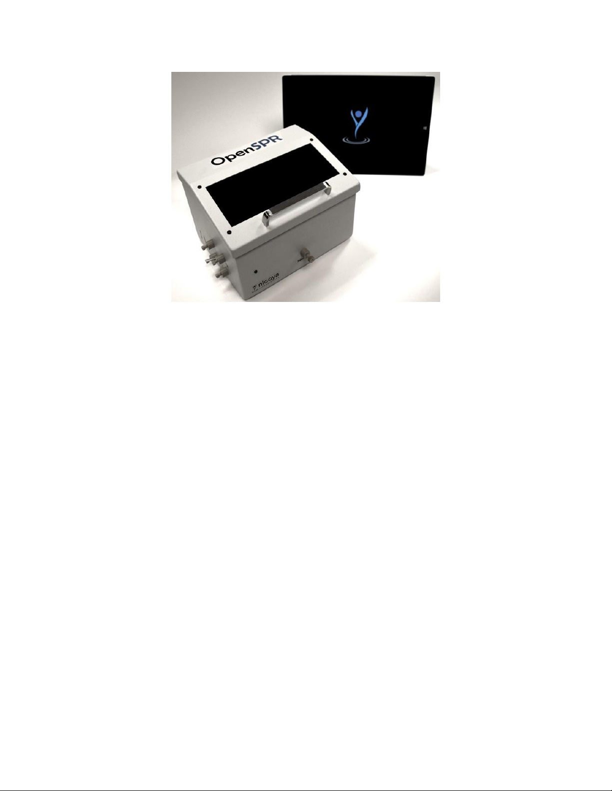
5. Switch on the OpenSPEC™power switch located at the back of the instrument [Figure 1.1].
The blue LED on the front of the instrument should turn on [Figure 1.2]. Start the OpenSPEC™
software by double clicking on the “OpenSPEC” desktop icon to connect the device.
Figure 1.1 - Back of OpenSPEC™ instrument contains connections for power and USB cables, and power switch.
Figure 1.2 - Front of OpenSPEC™instrument contains power LED and Injection Port.
Power Switch
Power Cable
USB Cable
Injection port
Power LED

9
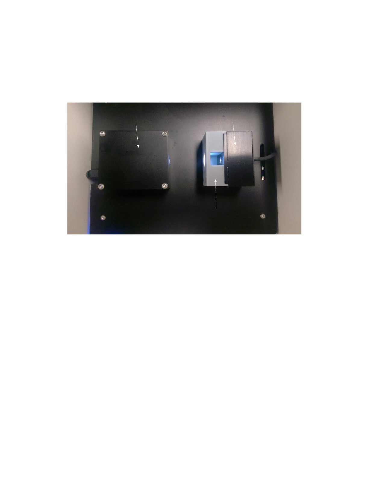
1.2 Overview of OpenSPEC™Instrument Components
The OpenSPEC™instrument consists of an optical detector (spectrometer), a light source, and a
cuvette holder [Figure 1.3]. There are also two temperature sensors within the instrument: one
on the circuit board (“Internal”) and one on the top plate of the instrument (“External”) (not
shown).
Figure 1.3 - OpenSPEC™instrument setup
Detector Light Source
Cuvette Holder

10
1.3 Operation Guidelines
1.3.1 Required Items
Computer with installed OpenSPEC™software
OpenSPEC™Cuvette Holder
Nitrile or Latex Gloves
1.3.2 Experimental Procedure
1. Ensure the OpenSPEC™ is connected to the computer and the power is ON.
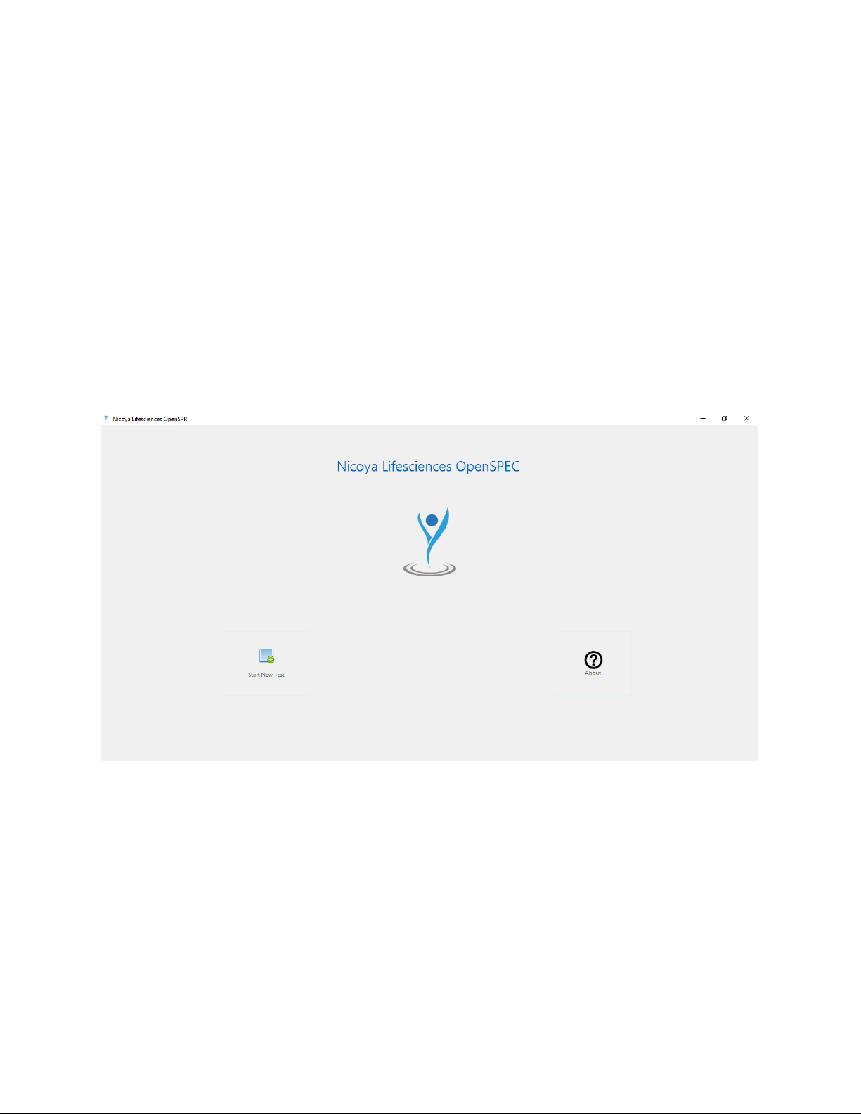
2. Open the OpenSPEC™ program on the computer by double clicking on the program shortcut.
The OpenSPEC™ Home Screen will open [Figure 1.4].
Figure 1.4 - OpenSPEC™home screen
3. Click the “Start New Test”icon.
4. A prompt will appear for selection of the destination where the test files will be saved [Figure
1.5]. The default location is in My Documents/OpenSPEC/TestResults. Next, chose a name for
the folder that will be created in which all data files will be saved. The date and time will be
automatically appended to the name.

11
Figure 1.5 - Select file destination prompt (left) and select folder name prompt (right).
5. Next, the hardware will connect to the software and the main Test Screen will open [Figure
1.6]. If the software does not connect automatically to the OpenSPEC™ device, an error
message will appear at the bottom of the screen. Ensure that the system is turned on and that
it is connected to the computer via USB. If so, click the reconnect icon in the top left corner of
the screen.
If the software still does not connect, a combination of turning the OpenSPEC™ device on and
off, unplugging and plugging the USB cable and restarting the software or computer may be
required. Always make sure the instrument is plugged in and turned on prior to starting the
software.
Figure 1.6 - Main Test Screen with highlighted reconnect button.

12
6. Once connected to the hardware, a new test can be started by clicking on the Start Icon in the
upper left corner.
7. The software will prompt you to take reference spectra.Thereference spectra include the light
and dark reference. Reference spectra consist of a Dark Reference and Bright Reference used
to calculate the absorbance. The Dark Reference is taken with the light OFF and the Bright
Reference is taken with the Light ON. It is best practice to take new reference spectra each
time a new test is started as this ensures the noise in the signal is as low as possible. However,
in some cases it is convenient to load a previous reference spectrum.
8. Select OK, and then choose whether to load a spectra saved from the last test, or take new
ones.
9. If you choose to take new references, the software will proceed to the below steps. If not, the
software will load the previous references and skill the section below.
Taking New Reference Spectra
1. OPTIONAL: In order to get the most accurate readings, you may want to subtract out the
optical properties of the cuvette holder and a reference liquid such as water. To do this, fill a
cuvette with water and place into the cuvette holder prior to taking the reference
measurements.
2. When prompted whether to use a previous reference spectrum, select “No”.
3. The system will first take a dark spectrum with the LED off. Then, the LED will switch on and
the instrument will automatically go through a number of conditioning procedures including
Warming Up, Checking for Spectrum Drift, and Waiting for LED to Stabilize.
4. Once the LED is stable, the software will capture the bright reference. You should now see a
red and blue line in the graph in the upper left corner of the software titled “Reference” that
look similar to that shown in Figure 1.7. The Red line is the Bright reference and the blue line
is the Dark Reference.
Figure 1.7 - Reference window: Red line is the bright reference, blue line is the dark reference.
5. Once the references have been taken, or a previous reference has been loaded, the software
will display a line in the graph in the bottom left of the screen entitled “Absorbance”. Without

13
any sample in place, the absorbance spectrum should be a flat line at an absorbance of zero
[Figure 1.8].
Figure 1.8 - Absorbance graph without a sample loaded. A flat line should be displayed.
If this graph does not display a flat line and the “Reference” graph looks good, retake the
Bright Reference by clicking the “Bright” icon near the upper left corner of the software.
If the integration time is higher than 1000 µs, or the “Reference” graph does not look
right, close the software and restart the test to take new references. Alternatively, both
reference spectra can be retaken manually. To retake the spectra manually, first, ensure
no Sensor Chip is loaded and the Flow Cell is clean and dry. Turn the LED off by right-
clicking on the “Dark” icon. When it is off, left-click on the “Dark” icon to take another
dark reference. Proceed to turn on the LED by right-clicking on the “Bright” icon. After
waiting for several minute for the LED to warm up, right click on the “Bright” icon to take
a new bright reference spectrum.
Loading a Sample
1. Once the reference have been completed, you will be asked to load your sample into the
cuvette holder.
2. Insert a cuvette into the cuvette holder. Ensure that the cuvette is inserted such that it is sitting
on the base of the cuvette holder and is in the proper orientation [Figure 1.9]. The orientation
of the cuvette is typically indicated by a triangle along the top edge of the cuvette. Ensure the
face of the cuvette containing the triangle is facing towards the detector. Ensure that the
cuvette holder is secure.
3. Fill the cuvette with at least 750µL of your sample solution (note –this will depend on the exact
type of cuvette used). The sample must completely fill the optical path. Also, you should
ensure your sample has an absorbance between 0.1 and 1 OD for optimal performance.

14
Figure 1.9 - How to properly insert a cuvette into the cuvette holder
4. You should now see the absorbance spectrum of your sample appear on the Absorbance
graph. Select OK to proceed.
5. The software will now prompt you to begin data fitting [Figure 1.10], in which the optical
spectra is fit and the peak position plotted in the Response graph on the right hand side of
the window. Select “Yes” to begin automatic data fitting.
Figure 1.10 –Ready to begin data fitting prompt
6. Once the fit is complete a green line should appear at the peak position on the Absorbance
graph and the data will begin to be plotted in the Response graph on the right hand side [Figure
1.11].

15
Figure 1.11 –Plotting of the peak position in real time
7. If the software cannot optimize the algorithm to find the peak automatically, you can manually
adjust the algorithm’s fit parameters in the “Parameters” tab in the ribbon bar as described
below.
Optimizing Peak Tracking Manually
Click on the “Parameters” icon to open a menu that will allow manual adjustment the settings
used to track the absorbance peak position [Figure 1.12].
Figure 1.12 Parameters menu.

16
The peak tracking works by fitting a Gaussian curve to the portion of the peak specified. The Fit
Parameters that can be adjusted include the Absorbance, Sharpness, Fit Width and Fit Index,
which are explained below:
Absorbance
Determines the minimum absorbance cutoff that the fitting algorithm will
use to find your peak.
Sharpness
Determines the minimum cutoff for the peak sharpness that the algorithm
will use.
Fit Width
This value determines the number of spectral points that the fitting algorithm
will use to fit the peak. There are approximately 2 spectra points acquired for
each nm in the spectrum.
Fit Index
This value dictates the peak index that with fitting algorithm will track. A fit
index of zero will track the peak present at the lowest wavelength.
An example procedure for manually fitting the peak in Figure 1.13 is provided below:
1. Start by changing the Absorbance Valve, which is indicated by the grey horizontal line. In
this example the peak is at an absorbance of approximately 1, therefore the Absorbance
value should be set lower than 1 as the minimum cutoff. Here it is set to 0.5 so it will not
look for any peaks below this value.
2. Next, set the Fit Index. In this example, we only have one peak present so we want to set
the Fit Index to 0. If two peaks were present above the Absorbance cutoff value, and we
wanted to track the peak located at a higher wavelength, we would set the Fit Index to 1.
3. Now adjust the Sharpness. If your peak is fairly broad as in the example provided, set the
sharpness to a value below 1. In this example the sharpness is set to 0.80. The sharpness
value can be increased to exclude peaks that are broader than the one you are attempting
to track.
4. Adjust the Fit Width according to the approximate width of the portion of the peak you
wish to track. Keep in mind there are approximately 2 spectral points measured for every
nm. In the example provided, if one wanted to fit the Gaussian curve used to track the
peak between 550 nm and 600nm, a Fit Width of (600-550) x 2 = 100 would be used. It is
recommended to use a Fit Width of 50 or higher for curve fitting and tracking. Note that
the Fit Width used can also affect the noise level of the response signal –the noise will be
higher if the Fit Width is too high or too low.
5. With the parameters set, confirm that the proper peak is being tracked as indicated by
the green vertical line on the Absorbance graph and the peak position looks accurate.
6. If the proper peak has not been found, or the peak position appears inaccurate, fine
tuning of a combination of the Sharpness, Fit Index and Fit Width may be needed.

17
Figure 1.13 Example absorbance spectrum.
In the “Data Averaging” section of this menu, the user can also control which data is displayed in
the Response Window, the raw data or averaged data or both. The user can also set the number
of raw data points used to produce the averaged data.
Recording events
If you would like to record an injection of a sample or other event, you can click the “Inject”
button in the ribbon and enter pertinent details regarding the sample, as shown in [Figure
1.15]. A marker will appear on the response graph, and will save the absorbance spectrum at
that point. The marked point will also be saved in the data file.
Figure 1.14 –Injection marker to record experimental events

18
1.3.3 Other Software Features
The graph windows can be resized by clicking and dragging the borders between the windows.
Double right clicking on any of the windows will open a menu that will allow the user to save an
image file or a .csv file of the data presented at that time. Double right clicking on the Response
Window will open a menu that will allow the user to change the x- and y- axis scales in a variety
of ways to better view the real-time data. See section “Adjusting the Response Graph” for more
details.
The bottom of the screen shows a message log that displays all changes made by the user to the
system during the experiment and reports the status of the instrument. If an error should occur,
it would be reported to the user here in red lettering. Everything printed in the message log is
recorded into the experimental Log file. At the top of the screen is the tool bar that allows the
user to control various experimental settings.
The OpenSPEC™ software tool bar [Figure 1.15] contains all the controls that the user may exploit
before and after an experiment. Each of these features are listed and explained below, from left
to right.
Figure 1.15 - OpenSPEC™ software tool bar.
Start/Finish Flag –This icon begins and ends the experiment. The user will be directed to
carry out specific tasks to conduct an experiment once it is clicked upon. Once the Finish
Icon is clicked, the software will no longer record any data.
Reconnect –This is highlighted when the software is having difficulty connecting to the
computer. The user should ensure that the instrument is on and properly connected to
the computer then click on this icon.
Bright and Dark Manual Reference –The lightbulb icons can be used to manually take
reference spectra for the instrument. When the user right clicks on the Dark icon they can
manually turn the LED off. When the user right clicks on the Bright icon they can manually
turn the LED on. To take a manual bright spectrum, the user must first manually turn the
LED on. The spectra taken will be displayed in the Reference Window. These spectra are
automatically determined before a test is conducted after the Start icon is clicked so
manual measurements are usually not necessary.
Integration time (µs) –The optimal integration time is automatically determined when
the Start icon is clicked so manual control of this number is not necessary. The user can
manually adjust the CCD readout frequency, thus controlling the amount of light that
reaches the CCD. Too much light will saturate the CCD, too little and the sensitivity of the
readings will be limited. When the user takes a bright reference spectrum after setting

19
the Integration time, they will see if the signal is saturated. The usual range of integration
times lie between 300 µs and 700 µs.
Boxcar Width –The boxcar width averages a single data point with the points around it,
thus smoothing the spectrum. This value is automatically set to 15, and must be set prior
to starting a test –it cannot be changed after a test has begun.
Scans to Average –This is the number of spectral acquisitions that the program will take
before displaying them. This value is automatically set to 20, and must be set prior to
starting a test –it cannot be changed after a test has begun.
Elapsed Time –This counter displays the amount of time that has passed during the
experiment. It can be converted from seconds to minutes and vice versa by right clicking
on the value.
Since Last Injection –This counter displays the amount of time that has passed since the
user last clicked on the Injection Icon. It is useful when the user is performing regimented
injections. It can be converted from seconds to minutes and vice versa by right clicking on
the value.
Sample Frequency (ms) –This is the amount of time that passes between spectral data
points recorded by the program. It is automatically set to 250 ms or 4 points per second.
Setting the value to 1000 ms would be one data point saved per second.
Parameters –Clicking on this icon will open a menu that will allow the user to manually
adjust the settings used to track the absorbance peak position [Figure 1.16]. The user can
also control which data is displayed in the Response Window, the raw data or averaged
data or both. The user can also set the number of raw data points used to produce the
averaged data.
Figure 1.16 - Fit Parameters menu.

20
Auto Fit Data –Clicking on this Icon will cause the software to “find” the absorbance peak.
This is done automatically at the start of the experiment. This feature is only required in
the rare situation where absorbance peak stops being tracked mid test (perhaps due to a
bubble). It is not recommended that this feature be used during an experiment unless the
absorbance peak is lost by the software which is signified by the disappearance of the
green line from the Absorbance Window.
Temperature –OpenSPECTM has 2 temperature sensors, one on the circuit board
(“Internal”) and one on the top plate (“External”). Temperature values from each are
recorded in the Test Results file.
Close –This Icon will close the screen and exit to the home page
Adjusting the Response Graph
The Response graph axis are defaulted to autoscale as the signal changes. However, it can be desirable
to zoom in or out on certain areas of the graph as test progresses.
The graph can be moved in the x and y axis by holding the right mouse button and dragging
the mouse.
The graph can be zoomed in and out by holding the middle mouse button and selecting a
boxed area to zoom in to.
The axes of the Response window can be adjusted to view the data better by double right
clicking on the graph. A menu will open with a number of options [Figure 1.17].
Figure 1.17 - Graph options menu that appears by double right clicking on the graph.
Reset Graph –Clicking this will return the graph to its previous settings. For example, if you
zoom in on the graph and want to return to your original view, click “Reset Graph”. This can
be especially helpful if it appears the graph is not updating.