Ostec IROS 05 TU User manual

IROS 05
IR Fourier Spectrometer
Operating Manual
FSVE.443430.005RE
© 2020 Ostec-Instruments, Moscow

This operating manual describes the technical specifications and operating principles of
Fourier Spectrometer IROS 05 (hereinafter, the spectrometer).
The spectrometer may only be operated by the specialists, who have read this manual,
are qualified to work on electrical devices up to 1 000 V and briefed on workplace safety rules.
The spectrometer involves operations with hazardous 220 V 50 Hz currents, as well as
hazardous and harmful chemical compounds.
The spectrometer operations should be governed by the following documents:
•Form FSVE.443430.00SFO
•Operating Manual FSVE.443430.00SRE

TABLE OF CONTENTS
Intended use, operating conditions, specifications, composition ....................................1
Spectrometer operating principles and exterior ...............................................................3
Operating principles ..........................................................................................................3
Spectrometer exterior .......................................................................................................5
Intended use.......................................................................................................................6
Before turning on ..............................................................................................................6
Device software installation..............................................................................................6
First run .............................................................................................................................7
Spectrum recording ...........................................................................................................7
Spectrum reading and copying..........................................................................................9
Spectrum identification ...................................................................................................12
Viewing spectra ...............................................................................................................15
Spectrum editing .............................................................................................................18
Calibration .......................................................................................................................19
Creating and editing libraries ....................................................................................20
Troubleshooting.........................................................................................................21
Spectrometer calibration .................................................................................................23
Maintenance, storage, and transportation .....................................................................26
Device accessories: built-on Attenuated total Reflection (ATR) and Specular-Diffuse
Reflection (SDR) block......................................................................................................27

1
Intended use, operating conditions, specifications,
composition
The spectrometer is intended to record infrared (IR) spectra of solid, liquid and gaseous
substances, including narcotic drugs, varnishes and paints, oil products, explosives,
pharmaceutical compounds. With add-ons and cells, the spectrometer also registers the
spectra of diffuse and specular reflections, as well as single and multiple attenuated total
reflection (ATR and HATR). A wide band IR microscope used as a spectrometer add-on helps
register the spectra of samples with linear dimensions of a few microns and above.
The spectrometer software helps perform quantitative and qualitative analysis of
received spectra, print, process and carry out other activities with them.
Full spectrometer name: Fourier Spectrometer IROS 05 TU 4434-801-59962935-08.
Please, see spectrometer operating conditions in Table 1. Spectrometer's
electromagnetic interference resistance complies with GOST 30804.6.1-2013, and radiated
interference with GOST 30804.6.3-2013.
Table 1. Spectrometer operating conditions
Parameter
Allowable bandwidth
Operating bandwidth
Ambient air temperature
10-35°С 15-25°С
Relative air humidity ≤80% at 35
°С 50-80%
Atmospheric pressure
84-117 kPa 97-105 kPa
Mains voltage
198-242 V 210-230 V
See the spectrometer scope of supply in Table 2, its technical specifications in Table 3.
Table 2. Spectrometer scope of supply
Name
Designation
Q-ty
IR Fourier Spectrometer
FSVE.443430.005
1
Software CD
ZalR 3.5
1
USB cable
1
Mains cable
1
1.25 A fuse element
2
Packing bag or box
1
Operating Manual
FSVE.443430.00SRE
1
Form
FSVE.443430. 00 5FO
1
When supplied with an IR microscope as part of a spectrometric complex, the Fourier
Spectrometer is provided with an additional set of adapter lenses for aligning with the
microscope.

2
Table 3. Spectrometer specification
Parameter
Value
Wavenumber operating range (with the ZnSe beam splitter for high
humidity operations) 550-5500 cm-1
Zero level limits
480-5700 cm
-1
Peak position measurement error
Systemic
±0.05 cm-1
Random
±0.02 cm-1
100% pass-band absolute deviation from 100% at
a resolution of 4 cm-1, triangular apodization, in 1
minute, in the following bandwidths:
600-800 cm-1
≤0.7%
800-2000 cm-1
≤ 0.4%
2000-2200 cm-1
≤ 0.2%
2200-2500 cm-1
≤ 2.0%
2500-3500 cm-1
≤ 0.4%
3500-5000 cm-1
≤ 0.8%
100% pass-band root mean square deviation (4
cm-1, triangular apodization, 1 minute) in the
following bandwidths:
550-650 cm-1
950-1050 cm-1
1950-2050 cm-1
3950-4050 cm-1
4950-5050 cm-1
Signal-to-noise ratio (RMS) in standard conditions:
in1 min, at a resolution of 4 cm
-1
in full bandwidth of 2000-2200 cm
-1
40 000
Signal gain
1, 2, 4, 8
Resolution
0.5, 1, 2, 4, 8 cm-1
Scanning speed, spectra per minute
For 1 cm-1
≈12
For 4 cm-1
≈49
Operating mode setting time
≤30 min.
Continuous operating time
≥ 8 h
Mean time to failure
≥ 10 000 h
Service life
≥ 10 years
Power consumption
≤ 100 W
Dimensions
Length
375 mm
Width
335 mm
Height
200 mm
Fourier spectrometer mass, less add-ons
15 kg
External optical outlet for connecting devices that are installed
outside sample compartment
available
Device autotest
available
Device digital electronic interface type
USB
As required by GOST 26828-86, the spectrometer has the following mark-ups:
•Manufacturer’s name;
•Spectrometer type;
•Manufacturer’s serial number;
•Year manufactured;
•Instrumentation type approval mark;
•Control designations;
•Inlet and outlet port designations.

3
Spectrometer operating principles and exterior
Operating principles
In terms of its operating principles, spectrometer IROS 05 is classified as a modulation
spectrometric device. Instead of using optical dispersing elements (prisms, diffraction
gratings, etc.) to split the radiation into spectral components, devices of this class use an
optical moving element to modulate the radiation flow and then perform electro-
mathematical processing of the signal from the optical detector that records this modulated
radiation as an interferogram.
The modulator in spectrometer IROS 05 is a double beam misalignment resistant
scanning interferometer Double Cat’s Eye (Russian Patent No. 1552791 dd 1993). See the
spectrometer optical scheme in Fig.1.
Figure 1. Spectrometer optical scheme
The inlet optical system (2) converts the IR source (1) radiant energy into a convergent
annular beam and makes it focus on the inlet port of the interferometer (3) consisting on
spherical mirrors and a moving beam splitter.
The beam splitter is a zinc selenide plate with a special coating that partially transmits
and partially reflects incident light. After a series of reflections, each beam falls on the beam
splitter again. The beams interfere, return to the mirrors, which this time act as a converging
optical system, and leave the interferometer through the mirror center ports.
The mirror system (4) converts the light escaping from the interferometer into a parallel
beam that passes through the cell holder (5) and is focused on the photodetector (7) by the
parabolic mirror (6).
Each monochromatic spectral component of amplitude Biand wavenumber σiat the
interferometer inlet has a corresponding photodetector signal:

4
,
where xis the path difference. In this case, the modulation depth for all wavelengths
will be the same, while the modulation frequency is different for different wavelengths:
,
where Vis the moving element speed.
The energy flow δI, striking the detector within the interval from σto σ+ dσ, where dσ
is the device resolution limit, will equal to:
,
By integrating across the entire spectrum, we get the complete flow Istriking the
detector:
The energy frequency distribution and the flow variable component are related with the
Fourier transform:
The interferogram is recorded as finite number of signal values registered by the
photodetector and digitized with analog-to-digital converter (ADC). Analog-to-digital
conversion is done at equal intervals of the optical path difference intervals.
The path difference reference scale is generated in a reference channel that consists of
a HeNe laser, the interferometer optical path aligned with the IR radiated path, photodetector
and the ADC control pulse generator.
Monochromator laser radiation with a wavelength of λ= 632.8 nm, which corresponds
to the frequency ʋ= 15 803 cm-1, goes through the same optical path as operating IR
radiation and forms the sinusoidal interferogram recorded with a special detector.
The detector signal is then used to generate a sequence of command pulses following
at λ/2 intervals that ensure a sample rate of Δx= ½ ʋ.
The recorded digital interferogram sent to the computer where it undergoes an inverse
Fourier transform.
The cells and holders are installed in the compact sample compartment on the device
top panel.

5
Spectrometer exterior
Designations on the device photos:
1. the Power light
2. the Scan light
3. peripheral equipment connection ports
4. sample compartment
5. MCT detector compartment cover
6. spectrum recording control buttons
Note: The photo displays the device in basic configuration. See Section 6 for the additional
equipment included in the package.

6
Intended use
Before turning on
Release the spectrometer from its factory package carefully and without turning it
upside down. Open the cell holder and remove the items from inside the holder. Check the
contents of the device delivery as per Table 2. Check the device for any visible damage.
Place the device in its permanent operating position. This is to be an even horizontal
surface protected against vibration (a firm heavy table). Do not place it near any vibrating
devices, including a computer case (the latter is to be on a different table). Stabilize the
spectrometer by turning the support feet.
Connect the spectrometer to power. Make sure you use a grounded socket. The
computer has to be connected to the same switchboard and a grounded socket. Connect the
device and the computer with the USB cable that comes with the device. The 220 V power
connector and USB port are on the rear and the right sides. The Power switch on the rear
side of the device case near the 220 V power connector.
Device software installation
First, turn on the computer. Run setup.exe on the USB flash drive that comes with the
device {the file may have a different name; however, there are no other files on the drive).
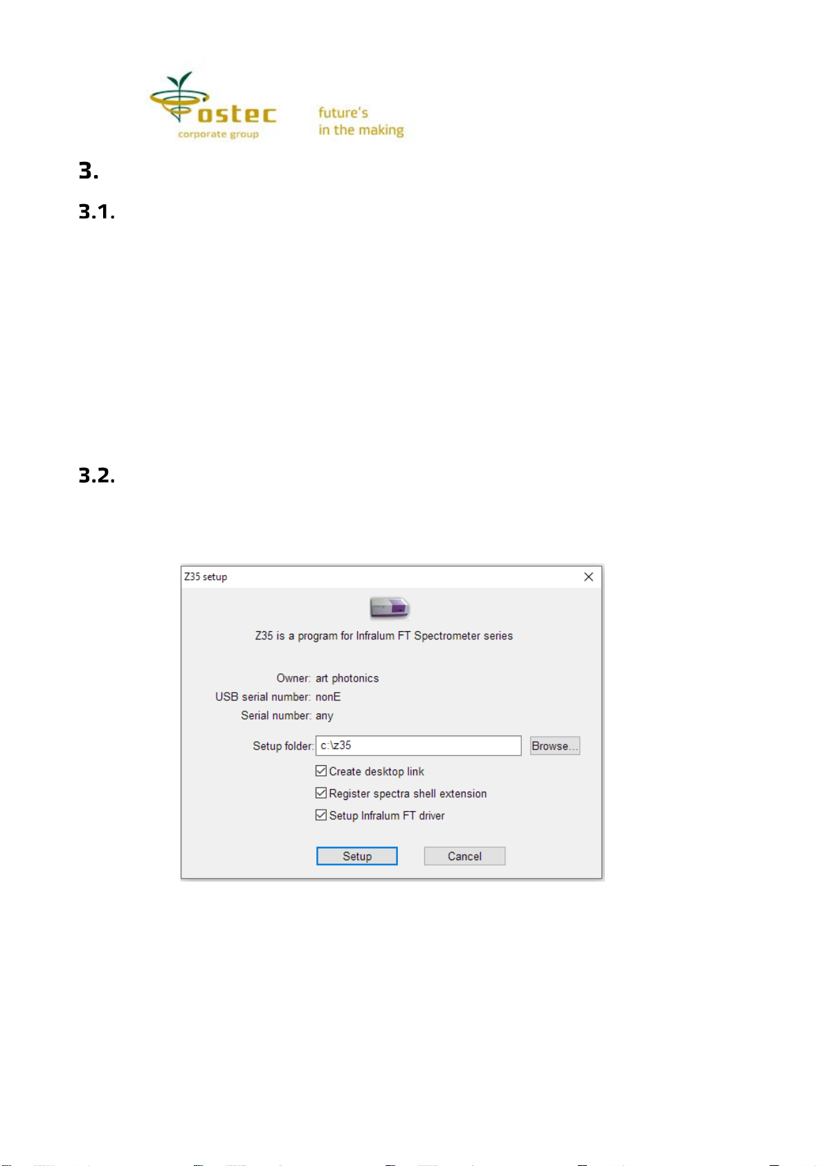
Specify installation conditions in the pop-up window {Fig. 2).
Figure 2. ZaIR 3.5 software installation settings
The installation folder hosts all the files required for operations. Additionally, the driver
components are copied to the operating system folders. The View spectra in the shell option
means that you will see the spectral images in the Explorer with the thumbnail view and open
them in ZaIR 3.5 by default.
As a rule, the software is updated by substituting the z35.exe file in the installation
folder with a new one. When updating through e-mail, you will receive a z35.exe module
already linked to your device. Unpack the archive and substitute z35.exe. If you have a
previous software version (z3.exe or zair.exe module), you will receive a setup.exe file that
includes all required components.

7
You may update your software through the Internet by clicking the Check for updates
command in the spectrum field context menu. You can also find this command on the User
Manual button menu. You can update the User Manual in the same menu.
ZaIR 3.5 supports Windows XP, 7, 8 and 10 operating systems. The gdiplus.dll module
may be missing in minor Windows versions. The module is included in the installation
software. If z35.exe fails to find gdiplus.dll, copy this file from the GDIPLUS folder to the
program-operating folder.
Use the standard Control Panel and Add and Remove Programs windows to remove the
device driver and software.
First run
Use the rear panel switch to turn on the device, the Power indicator on the front panel
will light green. In case the device driver was not installed at the first step (Section 3.2) or
the device has been off for a long time (a few days), Windows will ask to refer it to the IROS
05 device driver. Do not search for the driver on the Internet, choose automatic installation
and specify C:\z35\ FTD2XX as the file source path.
Run the device software. In a few seconds, the green Scan LED will start blinking on the
device case with a frequency of 1 time per second or less depending on the current spectral
resolution. The lighted LED means carriage forward stroke, dark LED means carriage return.
You can find a similar indicator in the bottom right corner of the software window. It is usually
a light blue circle that shifts right and left and right to indicate forward and return scans. The
triangular icons there indicate scan errors. Single errors can be caused by the device being
pushed or shaken. If errors keep occurring, or the LED on the case stops blinking, and the
software window indicator looks different from usual, it can mean device or software failure.
In this case, restart the program. If it does not help, unplug and again plug in the USB cable
or, in the worst case, turn off the device for a few minutes {see the troubleshooting section).
You can start recording spectra in 10 minutes after turning on the device and running
the software, we recommend that you start high precision measurements in an hour or later.
This is the time for the device to reach a thermal equilibrium. After changing the resolution,
you should also wait for a few minutes before you start recording.
Turn off the device for long idle periods {such as night). You have to turn the device off
before changing the computer or its parts, as well as before moving the device anywhere.
Spectrum recording
The main spectrum recording settings and commands are in the Record toolbar (Fig. 3).
The spectral resolution, or the minimum distinguishable distance between two peaks
can be set to 8, 4, 2, 1 or 0.5 cm-1. To do so, click the Resolution button and choose the value
you need in the menu. The current value is indicated on the button itself. Note that the
distance between spectral points is almost half the resolution value and is not divisible by it
but depends on the built-in laser wavelength (e.g., resolution 4 cm-1 corresponds to 1.93 cm- 1
between the points). The default resolution is 4 cm-1 that is used for the qualitative analysis
of organic compounds. The better the resolution, the longer are the scans and the lesser is
the green light flashing frequency.

8
The panel right shows the Number of Scans (or accumulations) set for spectrum
acquisition. If a scan (interferogram) meets the maximum position restrictions, then it is used
for spectrum calculation. The spectra for serial scans are averaged and the result is displayed
on the screen. Thus, the spectral image keeps updated until a required number of spectra is
accumulated (however, there can be more scans in case some of them are discarded). Larger
accumulations help reduce spectral noise. The noise does not show any significant changes
after 50 scans under ordinary conditions.
Figure 3. The main spectrum recording parameters and commands
If the Autorecord button is on, all spectra recorded on the device are automatically
saved on the drive under the name indicated in the File Name field. You can set any name in
this field. The default name is the current date and spectrum number. The spectrum is saved
in the folder that corresponds to the active list at window top of the software, the
corresponding line becoming selected. The current spectrum can be saved again under any
name using the Save spectrum command (the File toolbar).
Background spectrum. Before obtaining a sample spectrum, record a background
spectrum that will help take into account the impact of the atmosphere, fillers and other
recording conditions. If you introduce a sample using accessories (add-ons), put them in the
device cell holder without the sample only. Liquid cells are an exception: do not put one in the
device as the beams reflected from an empty cell distort the spectrum. Then click the
Background Spectrum button or press Shift+F9.
The spectrum recording time is proportionate to the number of the scans and can take
a few seconds. Meanwhile the window displays a spectrum for the actual number of
accumulations, the number being shown in the status bar (the bottommost of the program
window).
The obtained background spectrum is displayed in the window in a typical bell form.
Further, sample spectra will be divided by the background spectrum, which will help eliminate
the recording environment effects. You can use a previous background spectrum recording as
a reference spectrum. To do so, read the spectrum, then right-click on the spectra field and
choose Record →Use as background spectrum in the context menu. This is usually done if
you cannot restore the background recording conditions. As the number of points in a
spectrum depends its resolution, each resolution requires its own background spectrum.
When you select a resolution and an appropriate background spectrum has already been
obtained and recorded, it will load and apply automatically. If you try to obtain a sample
spectrum without a background spectrum, the program will prompt that you need first to
obtain a background spectrum.
Sample spectrum. Prepare your sample, put it in the cell holder and click the Sample
Spectrumbutton or press F9. The spectrum accumulation progress is displayed in the
window until you get a required number of scans. As a rule, you can set a smaller number of
scans than that for a Background spectrum. The sample spectrum is automatically cropped
by the frequency band previously set in the recording settings.

9
Device signal. The spectrum recording technique only involves the Current
Transmittance Spectrum option available in the button drop-down menu. If the option is
on, you can monitor the sample spectrum changes online and choose the recording spectrum
that fits your needs.
Note: You can also find the Background Spectrum, Sample Spectrum and Current
Transmittance Spectrum control buttons on the device top panel and use them instead of
the software buttons. Button colors: black for the Background Spectrum, yellow for the
Current Transmittance Spectrum, green for the Sample spectrum. The device will indicate
the current operating mode with an LED light flashing above the relevant button on the case.
Microscope (or Add-on... ) Switching to microscope, add-on and other peripheral
equipment operating modes. The device button has a relevant icon on it. If you use this
equipment, turn on a relevant option to operate them. To choose different equipment, click
the narrow triangle to the right of the button and select you add-on from the list. Note that
the scan number, resolution and other recording settings apply to the current selection, so
switching to another add-on will change some settings.
Recording settings. The button under this name displays a settings window, once you
set up your device these settings, as a rule, do not often change. These settings are described
in the User Manual that you can open by clicking a relevant button or a menu command in the
program.
Spectrum reading and copying
A spectrum saved on the drive can be read, searched, edited, and used for other
purposes. The usual way is clicking the spectrum reading command (a button on the File
toolbar) in standard operating system windows.
You can also open a spectrum from the lists at the program window top (Fig. 4). To do
so, double click your line or select the line with the mouse or navigation keys (arrows, PgDn,
PgUp, Home, End) and press Enter or Space. An open spectrum in the list is highlighted in a
different background color. You can open a maximum of 16 spectra at a time. To close a
spectrum, double click its line again, or press Enter or Space again.

10
Figure 4. ZaIR 3.5 software window
Each list also has a Read on the fly option (the button with a butterfly icon). If it is on,
the spectrum opens immediately after you select the line a closes when the selection shifts
to another line. In this case, if you want to open two or more spectra, select them with the
Ctrl (to select non-adjacent lines) or Shift (to select a continuous sequence of lines) key
pressed. On the fly reading activates by default for search results, you can also use it for
reading library contents.
All key strokes go to one active list. The active list window is highlighted with a thin
frame and a current line is marked with a dashed rectangle. Click on a window to activate it.
The Tab key switches to the next list. In addition to spectra, the lists can contain folders and
spectrum libraries. If you open a folder or library, the list will display the spectra in them.
The One level up button takes you to the previous folder level. The Home button takes
to the root folder of the particular list. You can make any folder a home folder by opening it
a clicking a context menu command.
Thus, you can navigate the folder system on the disk through the list. You can also open
logical spectrum folders: these are search results and search libraries. To do so, use the
Address text field above the list. This field has the full path to the currently open folder or
library. If you enter a different address in this field and press Enter, you will open the folder
at that address. You can display a drop-down folder list by clicking the button to the right of
the Address field. The first item on this list is the current folder, then all computer drives, and
then logical folders: search results and spectrum search libraries. The search results in the list
are for the sake of completeness. Selecting them from the list does not usually make any
sense as they open automatically after search, they do not have any results before that.
To return to the current folder after viewing search results, select the topmost line in
the drop-down list or click the One level up button. If a search library was open, One level up
will take you first to the search library list (this is another logical folder) and then to the
current folder.

11
Logical folders also contain spectra but their view depends on the folder type. Each list
is shown as a table with columns of various content. E.g., the search results have a column
that show the match rate between the selected spectrum and sample, and the search library
list shows the number of recordings and the spectral band for them. You can choose columns
to display in the list. The column types are listed at the top of the list context menu (with the
visible ones ticked). You can use the table headers to change column width (by dragging the
border between the header elements), column order (by dragging the elements), sort the list
by a field (by clicking the filed header). The changes only apply to the table view of the current
type of an open folder. Folders are classified as general folders, libraries, search library list,
search results. Switching from one type of folders to another changes the table view.
You can change almost any text field of the table right in the table. To do so, select a
field press F2 or click with the mouse. The field will open for editing and a text cursor will
appear in it. You can select a field with the mouse or the right or left arrow keys. The general
rule is: if a current line is changed, then it is selected in full. Thus, you can have to click three
times to open a field: the first click selects the whole line (if it has not been selected), the
second click selects a field in the line, and the third click opens the field. The keyboard also
requires three steps: select the line (up or down arrow keys), select a line field (left or right
arrow keys), and open the field (F2).
You can change the text in an open field and press Enter or click outside the field to
finish your edit. Field editing is has some restrictions. Some fields are not editable: these are
file creation time, search result match rate, and any fields in search libraries. Some file formats
(e.g., text, ASCII) do not support saving spectrum name and other parameters. The File field
is special: if you edit it, the file is renamed. As the Number field has the line number, entering
a number in this field results in the line under this number selected (e.g., you can use this
feature to get a spectrum from a library if you know its number). Table fields are helpful in
editing the names and recording settings of the spectra obtained with the device. After a new
spectrum is recorded, its name coincides with the file name and contains the spectrum number
and current date, which is not very informative. For this reason, you should change the
spectrum name right away and add some comments in the Conditions field. Remember that
a new spectrum is listed on the active spectrum list with its line highlighted.
You can drag and drop spectrum lists. That is you can pick a spectrum on a list with a
mouse click and drag it to another list, the desktop or any open folder on the computer. The
file with such spectrum will be copied to a relevant folder. Similarly, you can open any folder
on your computer and drag a file in it to a spectrum list. Libraries and search results act as
logical spectrum folders. If you pick a spectrum from a library {or from search results) and
drop it in a folder, you will create a JDX file in that folder and its name will consist of the
library name and the spectrum number in it. In addition, vice versa, if you drag a file to a
library, it will be supplemented with a relevant spectrum {unless it already has a spectrum
with the same name or the library is write-protected). You cannot drag recordings to search
results or directly from one library to another.
To add a spectrum to a library you can also use the Add to library command. In the
window, choose the library for recording {the drop-down list only has user libraries) and click
OK.
The ZalR software only provides for copying spectra by dragging, moving and deleting
are so far unavailable. To delete selected spectra, click the bin button above the list. By
deleting, you move spectra from the folder to the system Bin without additional prompts;
however, you can cancel it by clicking the Undo edits button. Deletion of files from the user
libraries cannot be undone, so the software asks for confirmation.

12
Spectrum identification
ZaIR 3.5 allows for identifying compounds by their IR spectra, name or other data by
searching the spectrum libraries (libraries are not part of the system and are supplied
separately). Click on the Spectrum Search button or press F5 to start searching an open
spectrum. In case of multiple open spectra, the first one is used. The search time depends on
the number of search libraries and computer capacity and does not usually exceed two
seconds. The button remains clicked during the search. If you unclick it before the search
finishes, the search will be suspended at the current phase.
The search results are displayed in the list on the left with the higher degree of similarity
to the searched spectrum at the top {the similarity degree is displayed in the Rate column).
While viewing the search results, the found spectra open as a second {red) curve.
Instead of search by a full spectrum, you can search by a part of it using the Search
bandwidth button. Clicking on it covers the spectral image with dark "curtains" that hide the
out of search spectrum sections. You can pick and move the curtains by dragging their edges.
Additional parameters are displayed in the Search Settings window that pops up after
you click the button with the same name. The Spectrum tab shows the maximum number of
the recordings to be selected and the minimum percentage of match rate. Peak positions and
heights to be considered are also set as a percentage of the maximum possible values. The
initial values are 85 and 25%, i.e. the peak positions are considered to a significantly greater
degree than their height, which helps identify spectra recorded under different conditions.
The Acceleration option involves all the CPU cores and multiplies the search speed almost by
the number of the cores. The Reset to initial values button restores the default values
applicable to ordinary tasks.
The other parameters under the tab refer to searching by mixtures. The command itself
is in the menu that drops down on clicking the side arrow to the right of the search button (in
other words, the button menu). Searching mixtures involves the ordinary search by spectrum.
The first entries of the search response, if their match rate is less than the preset value, are
searched again after substracting the spectrum from the query spectrum. As a rule, the preset
number of entries for a mixture search is smaller than that for an ordinary search (3–7) and
the rate is bigger {50–80%).
Note that a correct subtraction requires that the query spectrum be within the
absorption spectrum and reduced to it if it was in a different scale. Additionally, the spectrum
sections outside the absorption bands should be close to zero, otherwise the base line needs
adjustment. If it is not done manually, you should turn on the Subtract base line option. Note
that after an adjustment (including automatic) the spectrum is deemed changed and you will
be prompted to save the spectrum when closing it.
Turn on the Only mixtures option only in case you are sure that your sample is not a
pure substance. To eliminate results with single dominating substances, you can set the
minor component minimum content (the Component parameter).
Fig. 5 shows an example of mixture search for a mixture of two drugs. The search results
start with the spectra that are a linear combination of the library curves. Such an "artificial"
spectrum is marked with a"+" sign in front of the match rate. Click the sign to open the current
line for the other lines to display links to its substance components (the list on the left).

13
Figure 5. Mixture search results
The first line refers to the mathematically built mixture spectrum. The multiplier for each
component corresponds to its quantity in the mixture in relation to a pure sample. The total
of this multiplier can be unequal to 1. Further, the brackets contain a scaled component ratio
in %. You can see a good match between the total spectrum and the query spectrum. If you
take the spectra of the substances that comprise the total, then there will be a much worse
match, which is apparent from the match rate. Click the "+" sign again to hide the substance
component lines.
Select the Text tab to search by the name, element composition or other text attributes
of spectra. You can use the "*" sign for any letter sequence in your queries. E.g., if you enter
aspirin* in the name field, the search will return all names that start with aspirin, and *aspirin*
will return all names that contain the word in any position. The same applies to the Others
field. The Part of line option means that the * signs are added to the query line ends
automatically where they are not entered manually.
Use the B.F. field to mention all the element symbols indicating the number of each of
them or the range using a hyphen, e.g., C17 N3-5 02 Cl, note that you do not have to use 1.
Add * to your formula if you want it to include any other elements except the listed ones, e.g.
C17 N 02 *. Filling in several fields will return the compounds that satisfy all the restrictions
or, with Any field on, at least one of them.
You might not know the full sample spectrum but only the data on its absorption
bandwidth, e.g., the peak table. In this case, you should choose the Bands tab (Fig. 6). Use
one number to set the center of a bandwidth (peak) or two numbers with a hyphen to specify
the range, e.g. 1790-1810. Then you can specify your band intensity after a space (100% by
default). To switch to another line to enter a new bandwidth, press Ctrl+Enter (pressing Enter
alone starts a search). The Neighborhood field sets the maximum peak width in its height
calculation. The Min width means the peak position error margin if you only indicate its center.
Adjusted for height and Adjusted for width are specified as percentage of maximum. Their
initial values are 10 and 50%, i.e. height matters less than position.
If a library field contains peak data, then the search engine, with Form the peaks field
on, will use the peaks from the available peak table rather than from the spectrum curve. This
option, for example, works for UV spectrum libraries.

14
Figure 6. Peak (band) search conditions
Search for Mixtures only takes into account the peaks in the comparison spectrum. If
some of the query peaks are absent from the comparison spectrum, they do not affect the
general evaluation. This works if your query refers to a mixture and contains many peaks from
the different substance spectra. With the Mix option on, the spectra returned by the search
will be added in pairs in a proportion that provides for the best approximation to the query
spectrum. Such combinations are rated separately and added to search results in the form
shown in Fig. 5. You can apply mixing to any search but it works better for Search for Mixtures.
The following buttons are helpful with peak lists. Peak positions and widths are
displayed in the curve field after search: green bands for matching peaks, blue ones for the
others. If you click the View button, you can display them in advance. Use the Compare button
for comparison with the current spectrum and band coloring. Use the Purge button to
completely delete a peak list. The From curve button fills in the list again collecting peaks from
the current black curve in accordance with the selected threshold height. If you want to select
individual peaks only, move the cursor to the peak in your spectrum and when it is highlighted
with a dashed line, left-click on it. The peak will be added to the list and marked with a vertical
stripe on the image. Another click on it will delete the peak. Anyway, after supplementing your
list you can correct it manually.
If your peak table is typed or edited manually you should save it as a text file by clicking
the To file button so that you can read it later by clicking the From file button.
Use the Fragment tab to set structural formulas and their fragments for search; this is
only used if structural formula libraries are available. Methods of entering structures can be
found in the electronic manual.

15
The last tab, Library, is for setting the libraries for search. First, indicate the ones
available on the computer or local network. To do so, click the Add button, find the library file
folder, mark the files and click the Open button. The Delete button, on the contrary, excludes
marked libraries from the list (however, they are not deleted from the drive and can be added
later). Then mark the libraries in the list that will be used in your search (all items in the list
are marked by default). To mark more than one line, press Ctrl or Shift (just like in the
Explorer). The All button marks the whole list, and Inv. inverts your selection. The number of
selected libraries and spectra in them is indicated in fields Lib. and Sp. Note that the list
content coincides with the logical Libraries folder. When it is open in the list window, you can
add, delete, mark individual libraries for search using context menu commands the same way.
Viewing spectra
Each open spectrum in the spectrum field (program window bottom) has its own
sequence number and a curve color. By default, the first curve is black, the second is red, the
third is dark green etc. The status bar at the window bottom each curve has a corresponding
icon of the same color and number. Absent curves are marked with a dashed line. The
maximum number to display is 16 curves. You can change curve colors (and other properties)
through the context menu by right clicking above the curve or its icon. All operations (search,
edit) are usually performed on the first curve. The last open spectrum is marked as number 1,
the previously opened spectra are numbered in an ascending order by adding one. Any curve
can become number one if you click on it. You can also change the curve sequence by dragging
them to a new position. If the position is occupied with another curve, they will exchange
positions; if the position is empty, the curve will be duplicated. If you drop an icon outside the
status bar, the spectrum will close. You can also close a spectrum through its context menu.
The File toolbar can also be used to Close all spectra or Remove the last curve (i.e. the curve
with the biggest number). On the contrary, the Remember curve command copies the first
spectrum to the nearest vacant position.
Deletion, however, does not apply to invisible curves. An invisible curve does not show
up in the spectrum field and its presence is marked with a hashed icon. Double click the curve
icon or use the menu to turn invisibility on or off. You can use this function to protect a
spectrum against accidental deletion.
You can zoom in or out spectral curves. To zoom in a curve fragment drag the cursor
from the fragment top left to the bottom right corner with the left mouse button pressed. On
button release, the rectangle drawn will fill the window (Fig. 7). Drag from left to right only,
to expand your spectrum horizontally without changing the vertical scale. Similarly, move the
cursor from top to bottom to expand your spectrum vertically. You can scroll a zoomed-in
spectral image dragging it with the left mouse button or using the scroll bars. To return to a
full-scale image, drag the cursor from right to left with the left mouse button pressed.
Figure 7. Scaling curves with a mouse

16
You can zoom in and out using the green arrows on the View panel. They squeeze or
expand the spectrum scale along each axis separately. The Fit curve button change the scale
in a way fit the first curve in the window with a maximum zoom. A double click on a curve has
a similar effect, however, without changing the horizontal scale.
If the screen has more than one spectrum, they are all placed on the same horizontal
scale. By default, this is a wavenumber scale (cm-1), the numbers increasing from right to left.
You can change the direction by going to the context menu and choosing the X: left to right
option. You can switch the X scale to wavelengths {in microns) by clicking the Wavelength
button (unclick it to return to wavenumbers).
Unlike the X-axis, spectra can have different vertical scales and shifts for display
purposes. You can use the Same height option to compare spectra of various intensity. With
this option on, the vertical scale for the second and following curves is adjusted for all spectra
to have the same height. Additionally, each scale shifts vertically to align the bottom borders
of the spectral curves. The rule is named Align bottom. There are also Align top, Top to bottom
and Bottom to top alignment options when curves are placed one over another. Each curve is
in its own vertical scale in all these cases. If the spectra are on top of each other, the vertical
scales do not overlap and are drawn for each curve individually. When aligned by top or
bottom, the spectra overlap showing only the first spectrum scale. If you click on another
spectrum, it becomes the first and the vertical scale changes. However, by default, all spectra
show up on a common scale. All other variants are in the drop-down menu under the Common
scale button and can be selected explicitly (unless bottom alignment is enabled automatically
on selecting the Same height). Note that these variants do not affect the view if only one
curve is open.
Sample spectra can be displayed both in the transmittance scale {the quotient of two
spectra: current and background, for each point y=ys/yr,where index sis for the sample, and
rfor the background), and the absorption scale (decimal logarithm of this quotient with a
minus, y=lg(yr/ys)). Use the Transmittance button for switching. This switching does not affect
the Background spectra and interferograms.
All the properties described below are in the View section of the context menu, the
frequently used ones also show up on the View toolbar. Clicking on a small downward triangle
to the right of a button shows a drop-down menu that supplements the button command.
Overlay scale. The overlay dashed scale on a spectral image will not show up if you
unclick the Overlay scale button.
Peak captions. Clicking this button will add captions to sufficiently high peaks. The
sufficient height is shown with a red section in the image left field {the shorter the section,
the more peaks get captions). You can change the height by dragging the section bottom
edge or changing the number in square brackets near the edge (Fig. 8).
You can add a caption to a peak manually with a click on it. The peak must be selected,
and the cursor be a standard arrow (Fig. 8). If you click on a peak, it will be highlighted with
red lines, one solid at the base and two dashed ones: one shows the height and the other
shows the width at half height. You can shift the base edges, the height and width will remain
intact. For your convenience when moving the edges, the peak remains selected until the
cursor moves quite far from the peak border. The midpoint at the base moves vertically and
allows for changing the peak height only.
The peak captions at least include the peak X-axis position. The other properties, such
as width, height, area, can be added from the drop-down menu under the Peak captions
button or marked in the View context menu section. In the latter case, the changes in caption
will only apply to the selected peak.