AEA Technology, Inc. Bravo MRI II User manual

Dual Po
rt Vector Impedance Analyzer
rt Vector Impedance Analyzer
–
100KHz to 200 MHz

3
Proprietary Information.
Reproduction, Dissemination, or use of information contained herein for purposes other than operation and
/or maintenance is prohibited without written authorization from AEA Technolo y Inc. All ri hts reserved.
© 2003-
2014 by AEA Technolo y, Inc. All ri hts reserved. This document and all software or firmware
desi ned by AEA Technolo y, Inc. is copyri hted and may not be copied or altered in any way without the
written consent from AEA Technolo y, Inc.
VIA Bravo MRI II
TM
, Bravo PC Vision
TM
Patent No. 7,030,627 BI
Reproduction, Dissemination, or use of information contained herein for purposes other than operation and
/or maintenance is prohibited without written authorization from AEA Technolo y Inc. All ri hts reserved.
2014 by AEA Technolo y, Inc. All ri hts reserved. This document and all software or firmware
desi ned by AEA Technolo y, Inc. is copyri hted and may not be copied or altered in any way without the
written consent from AEA Technolo y, Inc.
TM
and AEA Lo os are trademarks of AEA Technolo y, Inc. 1998
Reproduction, Dissemination, or use of information contained herein for purposes other than operation and
/or maintenance is prohibited without written authorization from AEA Technolo y Inc. All ri hts reserved.
2014 by AEA Technolo y, Inc. All ri hts reserved. This document and all software or firmware
desi ned by AEA Technolo y, Inc. is copyri hted and may not be copied or altered in any way without the
and AEA Lo os are trademarks of AEA Technolo y, Inc. 1998

4
Bravo MRI II Operation Manual
AEA Technology, Inc.
Table of Contents
1 INTRODUCTION .................................................................................................................... 1
1.1 B RAVO MRI II H IGHLIGHTS ..................................................... 1
1.2 U SING T HIS M ANUAL .............................................................. 1
2 QUICK START ....................................................................................................................... 2
3 OPERATING THE BRAVO MRI II UNIT ................................................................................ 3
3.1 C ENTER F REQUENCY ............................................................. 3
3.2 S WEEP B ANDWIDTH ............................................................... 3
3.3 F REQUENCY S TEP S IZE .......................................................... 4
3.4 E XAM /P LOT ........................................................................... 5
3.5 P OWER O N ........................................................................... 5
3.6 P OWER O FF .......................................................................... 5
3.7 F1 H ELP S CREEN .................................................................. 5
3.8 F2 I NSTRUMENT P ROPERTIES (A DJUSTMENTSAND S ETTINGS ) .. 6
3.8.1 Backlight Control - Time/Intensity.............................................................................. 6
3.8.2 Display Contrast......................................................................................................... 6
3.8.3 Audio Options ............................................................................................................ 6
3.8.4 Cable Nulling.............................................................................................................. 7
3.9 F3 P LOT D ATA P ROPERTIES ................................................... 7
3.9.1 Left Plot Type (1
st
Plot) .............................................................................................. 7
3.9.2 Right Plot Data........................................................................................................... 8
3.9.3 RLC Model Series/Parallel......................................................................................... 9
3.9.4 Plot Width................................................................................................................... 9
3.9.5 Big Frequency Display............................................................................................... 9
3.9.6 Noise Filter................................................................................................................. 9
3.10 F4 S CALES AND L EGENDS ..................................................... 9
3.10.1 Grid Lines .............................................................................................................. 9
3.10.2 X Axis Label........................................................................................................... 9
3.10.3 Left Plot Scale ....................................................................................................... 9
3.10.4 Right Plot Scale................................................................................................... 10
3.11 F5 M EMORY AND M ISCELLANEOUS ....................................... 10
3.11.1 Save Operation.................................................................................................... 10
3.11.2 Recall Operation.................................................................................................. 10
3.11.3 Plot Name............................................................................................................ 10
3.11.4 Cable Impedance ................................................................................................ 10
3.11.5 Com Port Baud.................................................................................................... 11
3.11.6 Self Test............................................................................................................... 11
3.12 C ABLE N ULLING USING THE INCLUDED TERMINATORS .............. 12
3.12.1 Cable Definition ................................................................................................... 12
3.12.2 Nulling Procedure................................................................................................ 12
3.12.3 Calibration Cycles................................................................................................ 13

5
3.12.4 Numeric Quantities.............................................................................................. 13
3.12.5 80 Point Sweeps.................................................................................................. 13
3.12.6 100 Point Sweeps................................................................................................ 13
4 APPLICATIONS AND MEASUREMENT EXAMPLES ........................................................ 14
4.1 M AKE A ½ WAVELENGTH COAXIAL LINE .................................. 14
4.2 M AKE A ¼ WAVELENGTH COAXIAL LINE .................................. 14
4.3 L OAD C OUPLES INTO P OWER L INE ........................................ 15
4.4 T UNE AN ANTENNA TO RESONANCE ........................................ 15
4.5 M EASURE THE LENGTH OF A COAX ......................................... 15
5 OPERATION WITH THE VIA-RTD SOFTWARE................................................................. 16
6 CARE AND MAINTENANCE ............................................................................................... 17
6.1 O PERATING P RECAUTIONS ................................................... 17
6.2 E XTERNAL DC P OWER ......................................................... 17
6.3 B ATTERIES .......................................................................... 17
6.4 C LEANING ........................................................................... 17
7 LIMITED WARRANTY.......................................................................................................... 18
8 IN CASE OF TROUBLE ....................................................................................................... 19
8.1 C ONTRAST .......................................................................... 19
8.1.1 Environment and Contrast....................................................................................... 19
8.1.2 Power on Preset Value if Contrast Was Lost .......................................................... 19
8.1.3 Power Induced Failure............................................................................................. 20
8.2 B ATTERIES .......................................................................... 20
8.3 S ERIAL P ORT ...................................................................... 20
8.4 O THER P ROBLEMS ............................................................... 20
9 APPENDICES....................................................................................................................... 22
9.1 B RAVO MRI II S PECIFICATIONS ............................................ 22
9.1.1 Output Characteristics ............................................................................................. 22
9.1.2 Measurement Specifications.................................................................................... 22
9.1.3 Display Characteristics ............................................................................................ 23
9.1.4 Miscellaneous Specifications................................................................................... 24
9.1.5 Battery Power (choice of:) ....................................................................................... 25
9.1.6 Absolute Maximum Ratings..................................................................................... 25
9.1.7 Size.......................................................................................................................... 25
9.2 M ENU C HART ...................................................................... 26
9.2.1 Function Key Operations ......................................................................................... 26
9.2.2 Non Function Key Operations.................................................................................. 27
9.3 S ERIAL P ORT C OMMAND AND C ONTROL ................................ 28
9.3.1 Data Requests......................................................................................................... 28
9.3.2 Unit Setup................................................................................................................ 31
9.3.3 Examples................................................................................................................. 35
9.4 ASCII T ABLE ...................................................................... 36
9.5 C OAXIAL C ABLE R EFERENCE T ABLE ...................................... 37

1
1 Introduction
1.1 Bravo MRI II
Highlights
The Bravo MRI II analyzer measures complex impedances of electrical components,
Filters, antennae, and cables. The results of the measurements are displayed graphically,
with some numeric detail. You can choose to display the impedance from among several
formats. The Bravo MRI II sweeps across a range of frequencies, or operates at CW, either
way the display is continuously updated with new measurement results. This unit has many
applications, including:
1. Tune coils/antennae, filters, and feed systems
2. Measure Z, Angle, Resistance, and/or Reactance of a load
3. Measure Gain/insertion loss and phase of coupled circuits
4. Measure the length of a piece of coax
5. Portable and economic replacement for network analyzer applications that measure S11
and S21.
6. Find resonant frequency and response curve
7. CW signal generator
Two plots may be simultaneously viewed on the same graph. The Bravo MRI II connects
to your PC with the VIA-RTD Software to view results on a multi color, large screen display in
a Smith Chart or X-Y plot format.
The Z altering effects of coax cable can be nulled out, so that the load at the end of the
coax is displayed. The Bravo MRI II operates over a wide range of characteristic
impedances, so you are not limited to measuring 50 ohm systems.
The Bravo MRI II periodically self calibrates during operation when not in “Cable Nulling”
mode. The Bravo MRI II determines when recalibration is required and displays the marquee
screen with a “CALIBRATING” message during the calibration. The unit begins
measurements after a few seconds.
Operator conveniences include: non volatile storage, auditory cues, back lit display,
battery saver options, display contrast adjustment, versatile output displays, and serial port
communications. Internal Batteries (8 AA batteries, not included) power the Bravo MRI II in
situations where wall power is not available.
Included accessories are the VIA-RTD MRI Software, a power pack, a serial port cable,
and a soft case with shoulder strap.
1.2 Using This
Manual
Throughout this manual, references are made to FREQ and WIDTH keys. Each of these
keys has an UP or DOWN option. The operator selects the up or down keys depending on
desired results.
Certain words that appear as all capitals (FREQ, WIDTH, ON, OFF EXAM/PLOT,
ENTER) refer to keys on the Bravo MRI II keypad. Other capitalized “words” are acronyms
(VIA, SWR, CW, etc). Capitalized and italicized words (ENTER etc.) refer to keys on your PC
when using the VIA-RTD Software.
VIA is an acronym for Vector Impedance Analyzer, SWR stands for Standing Wave
Ratio, and CW is short for Continuous Wave.

2
2 Quick S t art
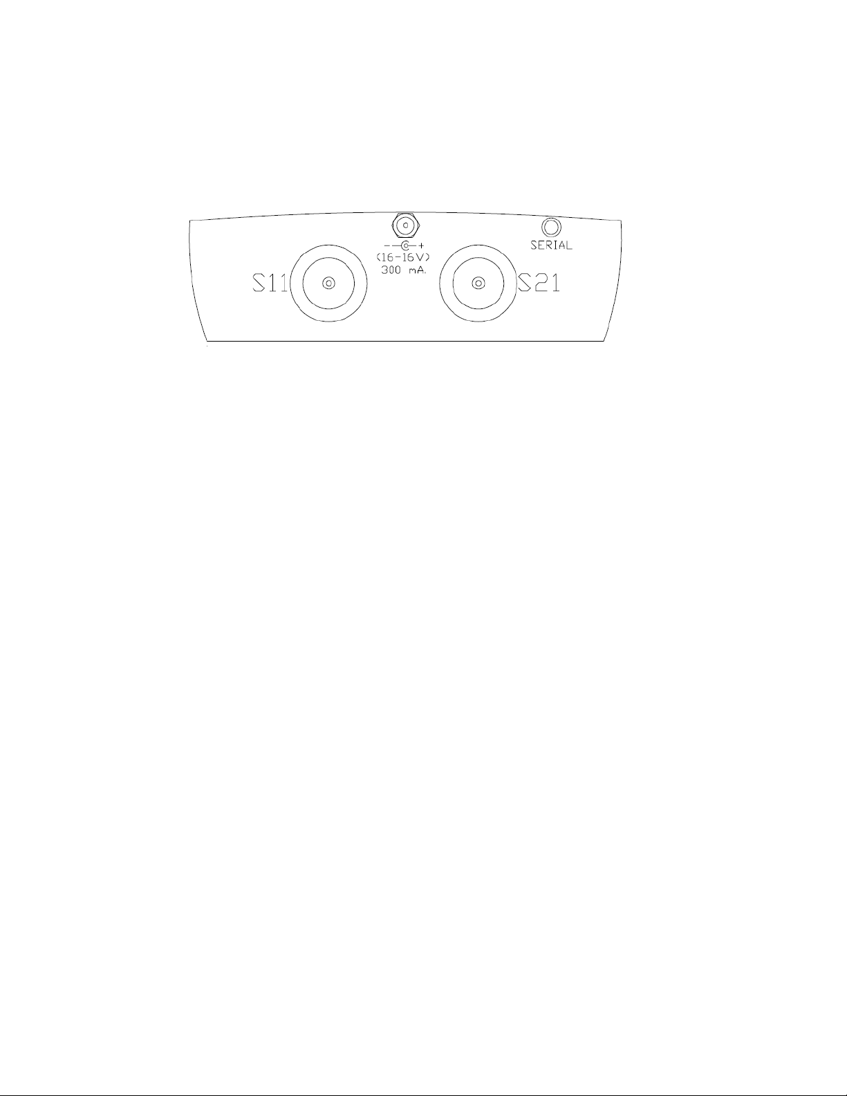
Connect the power pack to a wall outlet, the other end of the power pack plugs into the
jack located on the top panel of the Bravo MRI II, between the coaxial connectors. You may
optionally use batteries to power the Bravo MRI II.
Momentarily press the ON key. You should see the AEA marquee screen for a few
seconds, a calibration screen, and then a graph will appear. The factory default sets the
measurement type to S11 Vector mode, the left plot (thin line) to total Z (total impedance),
and the right plot (hashed line) to impedance phase angle.
An open circuit doesn’t make an interesting graph, so let’s connect a load to the S11
coaxial connector on the Bravo MRI II unit. A length of coax or a coaxial terminator would be
a good place to start. If you use coax, it will show a resonance at the half wavelength
frequency.
Enter a center frequency by pressing a number on the keypad (press the first digit of your
desired frequency). The screen changes to show the digit that you pressed. Press more
digits to until your center frequency shows on the display. Press the ENTER key when done.
Note: if you press a wrong digit, just add digits until you have an out of range frequency.
When you press enter, the frequency is erased and you can re-enter your frequency.
Now enter a sweep width by entering digits to get the desired width. Press one of the
WIDTH keys when ready. Due to synthesizer limitations, the sweep widths must be certain
values and the Bravo MRI II adjusts your entry to an available sweep width. The Bravo MRI
II flashes a brief warning if it changes the sweep width from the number you entered. The x
axis legend displays the lower and upper sweep frequencies.
Press the OFF key. The settings you have entered are automatically saved prior to the
unit shutting off. The next time you power up, these settings will reload, putting the Bravo
MRI II in the same state that you last used it in. If you ever want to start the Bravo MRI II with
factory preset values, hold the ENTER key while you power up the unit, otherwise, the unit
will load up the settings that were in effect the last time the OFF key was pressed..
Press the ON key again. Connect a load to the coaxial connector to measure its
impedance. Now press the EXAM/PLOT key. The plotting will freeze and a vertical cursor
appears. You may move the cursor with the FREQ keys. The two plot values at the cursor
frequency and the calculated L-C value are displayed by the three big numbers on the left of
the display. The top number shows the first (left) plot value, the middle number shows the
second (right), while the bottom number shows the inductance/capacitance of the load.
Using the FREQ keys, move the cursor to a frequency of interest. Pressing EXAM/PLOT a
second time returns to normal sweeping operation, with a new center frequency equal to the
last exam/plot frequency. See paragraph 3.4 for more details on EXAM/PLOT operation.
Refer to the remainder of the manual to find more operational details on these
and other functions.

3
3 Operating the Bravo MRI II Unit
You will navigate through various menus to control the operation of the Bravo MRI II.
Most menus operate in a similar manner. The top level menu is entered by pressing an F
key. The cursor on the left is scrolled to the desired choice by using the WIDTH or FREQ
keys. With the cursor aligned to the desired choice, press ENTER, and the first sub menu
appears. Again, use WIDTH or FREQ to scroll to the choice and press ENTER. Some sub
menus require different keys to operate, and this will be noted on the display.
A few functions require numeric entries instead of cursor movement. Enter the required
number using the numeric keys. Numeric entries set center frequency, sweep width, freq
step size, cable Z or cable VF.
Most menus will place the cursor at the current setting. So if you enter a menu by
mistake, you can usually press ENTER enough times to push through the menus without
altering the settings
Whenever you are in a menu, the Bravo MRI II lists your choices for keypad entries to
help you make your choice and return to measuring.
A table that shows the menu selections can be found in paragraph 9.2.
3.1 Center Frequency
Exit any menus that you may be in and then press the first digit of your desired center
frequency. The frequency entry screen pops up. Finish entering the center frequency. Note
that you may need to add zeroes to get your entry to align properly with the decimal point.
When the correct number is ready, press the ENTER key. The unit should start plotting with
the new center frequency.
You may also alter the center frequency using the FREQ keys. The center frequency will
shift up or down by the frequency step size. You are able to select the desired frequency
step size (see Para. 3.3).
If you make an error while entering the frequency, you can continue to enter digits until
an illegal frequency (too high) is entered. When you press the ENTER key, the display
resets, allowing you to start a new frequency entry.
3.2 Sweep Bandwidth
There are two ways to set sweep bandwidth, the first way is similar to center frequency
entry, except use WIDTH instead of ENTER; the second method is to just press WIDTH.
Notice that when you change the sweep width, the Bravo MRI II MRI will recalibrate itself.
Exit any menus that you may be in, then press the first digit of your desired sweep
bandwidth. The frequency entry screen pops up. Finish entering the sweep bandwidth.
Note that you may need to add zeroes to get your entry to align properly with the decimal
point. When the correct number shows in the display, press the WIDTH key. The unit should
start plotting with the new sweep bandwidth.

4
If you enter a width of zero, the unit will change to CW mode. Entering a non zero width
will convert the unit into sweep mode. The display formats are different for these two modes.
Another way to toggle these modes is explained in paragraph 3.8.4.
Due to synthesizer limitations, the sweep widths must be certain values and the Bravo
MRI II adjusts your entry to an available sweep width. For example if you enter a 1.000 MHz
wide sweep, the Bravo MRI II sets the sweep width to 1.000 MHz if the unit is plotting 100
points, but will set the sweep width to a 1.600 MHz if the graph is set to 80 points. The Bravo
MRI II flashes a brief warning if it changes the sweep width from the number you entered.
The x axis legend displays the lower and upper sweep frequencies of the chosen sweep
bandwidth.
Sweep width may also be set using the WIDTH keys. Pressing one of these keys will
increase or decrease the sweep width by a factor of 2. The WIDTH key may be pressed The
WIDTH key may be pressed and held for larger changes. Release the width key after the
desired number of beeps (each beep represents a factor of 2). If the width key is not held,
but is repeatedly pushed, you will have to wait for a calibration cycle to finish for each sweep
width.
Some combinations of center frequency and sweep width will cause the graph to be
truncated. The sweep truncates at the Bravo MRI II’s frequency limits. Truncation can also
occur using the EXAM/PLOT mode, see paragraph 3.4 for details on this.
If you make an error while entering the sweep width, you can continue to enter digits until
an illegal width (too wide) is entered. When you press the ENTER key, the display resets,
allowing you to start a new sweep entry.
3.3 Frequency Step Size
The frequency step size determines the change in center frequency when the FREQ key
is pressed. The center frequency will be adjusted up or down by using the appropriate FREQ
key. Setting the frequency step size is similar to center frequency entry, except use FREQ
instead of ENTER.
Exit any menus that you may be in then press the first digit of your desired step
frequency. The frequency entry screen pops up. Finish entering the step frequency. Note
that you may need to add zeroes to get your entry to align properly with the decimal point.
When the correct number is ready, press either FREQ key. The unit should start plotting with
the new center frequency. Any future presses of the FREQ keys will increment the center
frequency by this new step size.
If you make an error while entering the step size, you can continue to enter digits until an
illegal step (too big) is entered. When you press the FREQ or ENTER keys, the display
resets, allowing you to start a new step size entry.
The frequency step sizes are limited by the sweep parameters. If you enter an unavailable
step size, the Bravo MRI II flashes a brief warning and sets the step to a valid value as
close as possible to the step size you selected.
EXAMPLE: My unit was set at 75.3 MHz with a step size of 15 MHz. I wanted to step up
at 1 MHz increments, so I hit 1, 0, 0, 0, and then the Freq up-arrow. The synth required a
step size other than exactly 1 MHz, so it set it at 1.12 MHz. If I needed an exact frequency,
I can set it directly. In other words, if I needed to set the center to 76.3 MHz I would hit 7, 6,
3, 0, 0, and then ENTER.

5
3.4 Exam/P lot
The EXAM/PLOT key toggles between two modes of operation. In the plot mode, the
screen is periodically updated with the results of a new measurement. The exam mode
freezes the display, and adds a frequency cursor. The cursor shifts by pressing the FREQ
keys. The plot data values under the cursor are displayed numerically on the left edge of the
graph.
When the Bravo MRI II calibrates itself, it sweeps a bandwidth that is twice a large as the
display. This will allow you to do panning operations in the exam mode without triggering a
new calibration cycle. This expanded calibration width improves operator convenience when
panning, especially when using the cable null feature. To suppress the calibration cycle, only
press the FREQ key while in exam mode, pressing the FREQ key in the plot mode forces a
new calibration.
You may also press the ENTER key during exam mode. The cursor position determines
the new center frequency, and you will be back in plot mode.
If you pan far enough, you will notice that the graph truncates. The truncation occurs at
the edge of the calibrated frequencies. If you wish to remove the truncation, you must force a
new calibration cycle. One way to do this is to just enter a new center frequency (para 3.1). ).
Other ways to force a calibration cycle are to press the FREQ or WIDTH keys while in the
plot mode (para 3.1or 3.2).
EXAMPLE: Once you press the EXAM/PLOT key, the cursor comes up. Press the
FREQ down key until the cursor reaches the far left of the screen. Hitting EXAM/PLOT again
brings the unit back to PLOT mode with the new center frequency without re calibrating .
You can now hit EXAM/PLOT again and continue moving the cursor to the left.
3.5 Power
On
The unit is powered up by pressing the ON key. Be sure the power pack is connected or
that you have good batteries installed. The unit is configured with the settings that were in
effect when the OFF key was last pressed. If you ever want to start the Bravo MRI II with
factory preset values, hold the ENTER key while you power up the unit.
3.6 Power
Off
To turn off the unit, press the OFF key. The settings (center freq, sweep width etc.) are
automatically saved to memory prior to turning off. These values will be recalled the next tine
you power on. If you power down by merely unplugging the power pack, the present settings
will not be saved.
3.7 F1 Help
Screen
T he help screen displays an abbreviated overview of the function keys. This can be
used to figure out which menu something is located in without having to explore through the
menus.

6
3.8 F2 Instrument Properties (Adjustments and Settings)
This menu contains items that alter the physical properties of the Bravo MRI II unit.
3.8.1 Backlight Control - Time/Intensity
The backlight provides a convenient way to view the display when operating in dimly lit
locations. The life of the backlight (and the batteries, if used) can be extended by using the
backlight only when needed. You have control of the backlight operation. You may turn the
backlight on (continuous) or off. There are also 3 choices to turn the backlight on for a limited
time before it automatically shuts off. You can also adjust the backlight brightness from this
menu. Use WIDTH to move the cursor to the desired choice for the timer. Use FREQ to
adjust the intensity. When you have finished choosing your settings, press ENTER and you
will be back to measuring.
Note that the backlight turns on when you enter this sub menu. If you want to keep the
light on while measuring, the timer must be set to something other than “off”. When using the
timer (10, 20, or 50) any key presses will reset the timer function. If you have the backlight
set to 10 sweeps, the light goes out after 10 sweeps. If you press a key, the light will come
on again for another 10 sweeps after returning to measuring.
Also note the maximum intensity is limited and the backlight will only be noticed in dim
light conditions. When the Bravo MRI II is in a bright environment, the backlight will be
washed out.
The lowest brightness level is equivalent to the off setting. Either way of shutting off the
backlight will save the same amount of battery power. The brighter the backlight intensity,
the more battery power is used (if running off of the batteries).
3.8.2 Display Contrast
The display contrast can be affected by ambient temperature, so an adjustment is
included. Once in the contrast sub menu, press and hold the WIDTH or FREQ key until the
desired contrast appears. Press ENTER when done.
3.8.3 Audio Options
Pressing a key on the keypad optionally produces an audible beep. You may adjust the
volume level of these beeps. You may also activate an audio readout for when you want to
hear the effects of your adjustments rather than watching the display. In the audio readout
mode, the pitch of the audio varies as the left plot value at the center frequency changes.
Thus if you are measuring total Z on the left plot, the audio pitch gives an indication of the
total Z measured at the center frequency,
Once in the audio sub menu, press WIDTH to set the volume, or press FREQ to toggle
the audio readout mode. Press ENTER to leave the audio sub menu.

7
3.8.4 Cable Nulling
The Bravo MRI II Unit can operate with or without cable nulling. Enter this sub menu to
select which mode of operation you want. When you select the nulling option, the unit will
step you through the appropriate cable nulling routine depending on whether you are in S11
or S21 mode. You will be prompted to utilize the supplied Short and 50 Ohm terminators at
the proper times.
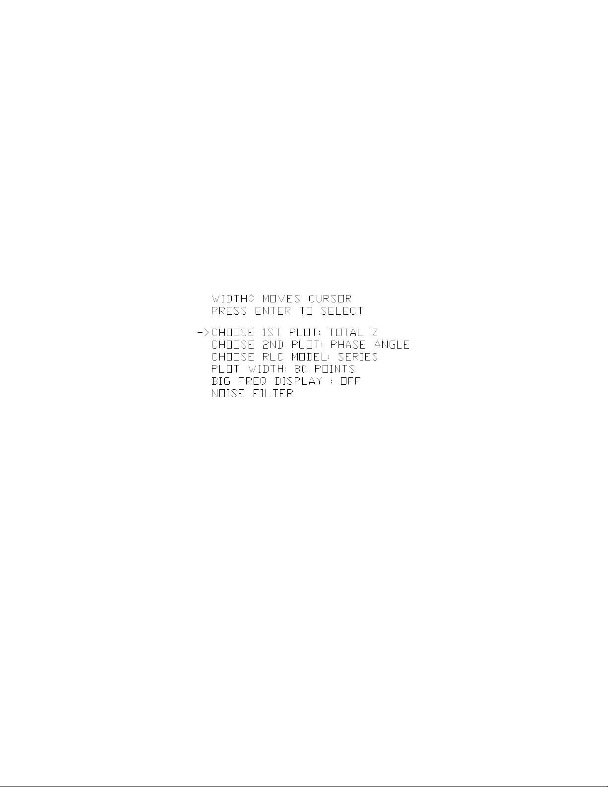
3.9 F3 Plot Data
Properties
The Bravo MRI II can graph up to two plots on the display. More plots may be displayed
if you connect the Bravo MRI II to a PC running the VIA-RTD software. In addition to the two
plots, some information is also displayed numerically. When the plotting width is 100 points,
all of the center frequency data is displayed with small digits. When the plot width is 80
points, the left plot and right plot values at the center frequency are displayed with large digits
(viewable from 8 to 10 feet). Additionally the 80 point sweep displays using large digits, the
calculated L-C (in VIA operation) or the Q of the SWR curve (in SWR operation).
3.9.1 Left Plot Type (1
st
Plot)
This sub menu allows you to choose which data to plot on the left axis with the non-
hashed curve. The data types depend on the instrument mode. The center frequency value
is also displayed numerically.
3.9.1.1 S11 O peration
3.9.1.1.1 Total Z
This is the total Z of the load. It is equal to the square root of the sum of resistance
squared and reactance squared. If resistance and reactance are made to be the two legs of
a right triangle, the total Z is the hypotenuse.
3.9.1.1.2 Z
Angle
The impedance angle is the ratio of resistance to reactance, expressed in degrees. It is
equal to the arctan of reactance divided by resistance. Note that this angle is a bipolar
quantity, so zero is near the middle of the plotting range, the x axis is down at the maximum
negative, and the maximum positive is still near the top of the plot.
3.9.1.1.3
Resistance
Standard resistance, measured in ohms. This is the portion of the Z that is non reactive.
3.9.1.1.4
Reactance
The reactance is the non resistive portion of the total impedance caused by capacitance
or inductance. Reactance is also a bipolar quantity, thus zero reactance is at the middle of
the plot range.

8
3.9.1.1.5 R.C. Mag (Reflection Coefficient Magnitude)
This is the magnitude of the S11 vector. Minimum value is zero and implies perfect
match. Maximum value is 1.0, complete reflection of energy.
3.9.1.1.6 R.C. Angle
(Reflection Coefficient Angle)
This is the same thing as the phase angle of the S11 vector. This angle contains the
information to determine cable length. Combined with the magnitude, all the impedance
information can be determined.
3.9.1.1.7 SWR
SWR is the same as voltage standing wave ratio. This can be used to roughly determine
an antenna’s match to its coax.
3.9.1.1.8 RTN
Loss
The amount of transmitted energy that is reflected back, expressed in dBs.
3.9.1.1.9 No Plot (self
explanatory )
3.9.1.2 S21 O peration
3.9.1.2.1 Linear
Gain
The returning signal into the S21 Port is measured in relation to the signal going out on
the S11 port, expressed in linear units. i.e. a measure of 1.00 means the incoming signal is
the same as the outgoing signal amplitude. (1 mW in for every mW out).
3.9.1.2.2 S21
Angle
The phase of the returning signal is measured in relation to the phase of the outgoing
signal, expressed in degrees ( + / - 180 degrees)
3.9.1.2.3 Log
Gain
The same measurement as Linear Gain, but expressed in dB’s. a logarithmic scale.
3.9.1.2.4 No
Plot
3.9.2 Right Plot Data
Any data available for the left plot can be plotted on the second plot. Even the same data
can be plotted on both plots (use different scales to see both). See paragraph 3.9.1 for
detailed information on plots. The curve of the right plot is always a hashed line.

9
3.9.3 RLC Model Series/Parallel
The equivalent L or C (calculated from the reactance at the center frequency) can be
displayed numerically. The equivalent load appears as a resistor and a capacitor (or resistor
and inductor). The values of the resistance and reactive component can be calculated as two
components in series or two components in parallel. Selecting series or parallel determines
which calculation is used when displaying resistance or reactance. This calculation (series or
parallel) affects both the numeric output and the plots for resistance or reactance. This
option has no effect on SWR plots, total Z, or impedance angle.
3.9.4 Plot Width
The graphs can be either 80 or 100 points wide. 80 points gives a smaller sweep range
with only 8 horizontal divisions, but it allows the large numeric display of center frequency
values. When 100 points are used, there are 10 horizontal divisions, and the KHZ/division is
easier to keep track of mentally because it is easy to divide by 10. However, the 100 point
display leaves no room for large numeric displays, so all center frequency values are
displayed with small digits. Pick the plot width you are most comfortable with.
3.9.5 Big Frequency Displa y
An option to display the center frequency with large digits is available. This option is only
available on the 80 point plot. This display does cover a portion of the plots so you
usually use it when covering a portion of the plot doesn’t bother you.
3.9.6 Noise Filter
A smoothing filter is available to reduce the unwanted effects of high frequency
interference such a gradient noise. Be aware that this filter works on ALL sharp curves in
a plot and may effect your readings in sharp curve plot areas. See example #1 at the
back of the manual.
3.10 F4 Scales and
Legends
This menu allows you to select the plot scales, the x axis format, and the number of
horizontal grid lines to show
3.10.1 Grid Lines
You can choose 1, 3 or 5 horizontal grids
3.10.2 X Axis Label
You can choose between 3 frequencies (FL FC FH) or the center frequency plus/minus
the delta frequencies (-dF FC +dF).
3.10.3 Left Plot Scale
Select the scale of the left plot. Choices vary depending on what is being plotted.

10
3.10.4 Right Plot Scale
Select the scale of the right plot. Choices vary depending on what is being plotted.
3.11 F5 Memory and Miscellaneous
This menu lets you save and recall data, set the plot name, set the cable properties, set
the baud rate, and perform a self test.
3.11.1 Save Operation
Instrument states and /or data may be saved in EEprom for recalling at a later time.
There are two types of save memories. The first type only saves instrument presets; the
other saves both the presets and the plot data. One can use the preset only memory to save
instrument states for a number of different antennae. The full data save could record the
impedance of an antenna then transfer it to a PC for further analysis or to save history
information.
3.11.1.1 Instrument Preset s
Memory locations 1 through 16 save the instrument presets only.
3.11.1.2 Plot Data
Memory locations 17 to 24 save both plot data and instrument presets.
3.11.2 Recall Operation
Memory recall is the compliment to memory save. When memory locations 17 to 24 are
recalled, the saved data is displayed, and the unit is in the exam mode, allowing you to view
the data and move the cursor across it. Once you leave the exam mode the display is
updated with new data, but the saved data is still intact in the save memory slot, ready to be
recalled again if necessary.
3.11.3 Plot Name
Allows you to assign up to a 12 character name to the save data. A descriptive name will
help you remember what the plots are when downloading the data to a PC. You can enter
the name via this submenu, or you can enter it during the save operation.
3.11.4 Cable Impedance
You set the cable Zo and velocity factor in this sub menu. Operation is similar to
frequency, you my need to enter zeroes to align the velocity factor to the decimal point. The
Zo is used for SWR calculations. The velocity factor is used in cable length calculations.

11
3.11.5 Com Port Baud
You can set the bit rate you wish to use in this sub menu. The data format is always N-8-
1 with XON/XOFF handshaking.
3.11.6 Self Test
You can perform a self test by selecting this choice. Press ENTER to quit the self test.
Pressing any other key creates a response that indicates the key is operating.

12
3.12 Cable Nulling using the included terminators
Any load connected to a coax that is not perfectly matched to the coaxial cable’s
characteristic impedance will have its impedance modified by the coax. Cable nulling allows
you to remove the effect of the coaxial cable so that the impedance you read shows the
impedance of the load at the end of the cable, without the cable modifying effects.
Cable nulling is selected by using one of the (with cable) options when selecting the
instrument mode. The Bravo MRI II will prompt you for the required action during the cable
nulling procedure. Basically, the Bravo MRI II takes three readings: open circuit, short circuit,
and nominal Z
0
.
The data that results from a procedure that nulls a cable will be specific for that cable. If
the cable is changed, a new nulling must be performed. If the power is turned off, the cable
nulling information will be lost, so a new cable nulling procedure will be required after power
is restored. Note, if you power-up again and do not wish to use cable nulling, you can just
fake it by going though the nulling procedure without any cable or load, then change the
instrument state to “no cable”.
3.12.1 Cable Definition
The coaxial cable characteristic impedance must be defined for cable nulling to operate
properly. This can be done in the Cable Characteristics sub menu (see 3.11.4 ).
3.12.2 Nulling Procedure
The nulling procedure begins by selecting a <with cable> option when setting up the
instrument mode (see Error! Reference source not found.or Error! Reference source not
found.). Install the cable to be nulled to the RF connector of the Bravo MRI II unit. Once the
instrument mode is selected and the cable is connected, the procedure can begin using the
included terminators.
3.12.2.1 Open Circuit Reading
With the far end of the coax un-terminated (open circuit) press the ENTER key once. A
few seconds later the Bravo MRI II will prompt you for the next reading…(a short).
3.12.2.2 Short Circuit Reading
With the far end of the coax shorted using the coaxial short, press the ENTER key once.
When this step is complete the display shows that it wants the nominal impedance
termination, usually 50 (or 75) ohms.
3.12.2.3 Nominal Z Reading
With the far end of the coax terminated with a matched load (50 Ohms is included in the
kit), press ENTER once. The firmware will compute and apply the corrections. This
completes the cable nulling procedure. To verify that you completed the procedure correctly,
notice that the display shows flat line(s) at Z
0
(and near zero degrees). If that procedure went
well, remove the matched load. Now you are ready to take measurements at the end of the
coax. If you do not see flat lines at the expected values, redo the procedure starting at
3.12.2.

13
3.12.3 Calibration C y cles
The Bravo MRI II MRI will periodically enter a calibration cycle. This ensures the best
accuracy over long periods of time. Changing certain sweep parameters can also induce a
calibration cycle. Sometimes you may want to enter something into the keypad while a
calibration cycle is in progress. This is allowed, so you may repeatedly bump the width or
alter the center frequency without waiting for the calibration cycles to finish. However after
you have completed your sweep alterations, the Bravo MRI II MRI performs one last
calibration cycle before displaying the new data.
3.12.4 Numeric Quantities
The Bravo MRI II compliments the plot displays with a number of numerical quantities.
These quantities depend on the sweep settings and the instrument mode.
3.12.5 80 Point Sweeps
The 80 point sweeps use large font numbers that can be read from about 10 feet away
with proper lighting/backlight conditions. The numbers are, from top to Bottom:
1. Left Plot center frequency value
2. Right Plot center frequency value
3. Q of Impedance plot if Z is plotted
3.12.6 100 Point Sweeps
There are 11 numbers listed on the left side in a small font. The numbers are, from
top to Bottom:
1. Z = Total Z
2. A = Z Angle
3. R = Resistance, or real portion of Impedance
4. X = Reactance, or Imaginary portion of Impedance
5. S = SWR
6. L = Return Loss
7. C = Reflection Coefficient Magnitude
8. A = Reflection Coefficient Angle
9. G = Linear Gain
10. P = Gain Phase
11. L = Log Gain

14
4 Applications and Measurement Examples
4.1 Make a ½
wavelength coaxial line
To make a coaxial line that is tuned to one half wavelength:
1. Start with a piece of coax that is slightly longer (about 5 to 10%) than calculated. The
formula for a ½ wave cable is:
L = 491(vf) / fr where
L = length in feet
vf = velocity factor (usually between .6 and .9)
fr = frequency.
2. Connect one end of coax to Bravo MRI II (preferably using a coaxial connector), the
other end is left open. Set the Bravo MRI II center frequency to the desired ½ wave
frequency. There should be an impedance peak (and a zero phase crossing) slightly to
the left of the center frequency. The zero phase crossing should go from upper left to
lower right. Use wire cutters to snip off small pieces of the coax from the unconnected
end. Every time a piece is removed, the zero phase crossing should move to the right.
When the zero phase crossing reaches the center frequency, the coax is at ½ wave
length.
3. Alternate method: Far end of coax is shorted. Look for zero phase crossing from lower
left to upper right. Impedance will be very low. This method is less preferred, as the
coax must be re-shorted after every snip.
4.2 Make a ¼
wavelength coaxial line
To make a coaxial line that is tuned to one half wavelength:
1. Start with a piece of coax that is slightly longer (about 5 to 10%) than calculated. The
formula for a ½ wave cable is:
L = 245.5(vf) / fr where
L = length in feet
vf = velocity factor (usually between .6 and .9)
fr = frequency.
2. Connect one end of coax to Bravo MRI II (preferably using a coaxial connector), the other
end is left open. Set the Bravo MRI II center frequency to the desired 1/4 wave
frequency. There should be a low impedance and a zero phase crossing slightly to the
left of the center frequency. The zero phase crossing should go from lower left to upper
right. Use wire cutters to snip off small pieces of the coax from the unconnected end.
Every time a piece is removed, the zero phase crossing should move to the right. When
the zero phase crossing reaches the center frequency, the coax is at 1/4 wave length.
3. Alternate method: Tune the Bravo MRI II to twice the ¼ wave frequency, and look for
the zero phase crossing (upper left to lower right).

15
4.3 Load Couples into Power Line
Occasionally, an antenna will strongly couple into nearby power lines (e.g. a long wire
antenna in the attic). When this occurs, the plot lines may be “thicker” and the readings will
shift around a lot. There are two methods to eliminate this effect
1. Power the Bravo MRI II from batteries. The wall power pack must be unplugged from
the Bravo MRI II power jack to do this.
2. Connect the ground sleeve of the coaxial connector to an earth ground.
If the above methods do not clear up the plots, there is most likely an interfering signal
causing the problem.
4.4 Tune an antenna to
resonance
To tune an antenna to resonance, set the Bravo MRI II center frequency to the desired
resonant frequency. Connect the Bravo MRI II to the antenna. Using the adjustment
provided by the antenna manufacturer, tune the antenna for a zero phase crossing at the
Bravo MRI II center frequency. The tuning adjustment could be one of several methods, and
should be mentioned in the instructions for the antenna.
4.5 Measure the length of a
coax
To find the length in degrees (at some frequency) set one of the plot types to Reflection
coefficient angle (see paragraph 3.9.1.1.6). Set the Bravo MRI II center frequency to the
frequency of interest. Note the RCA reading. By adjusting the sweep width to the widest,
and stepping through a number of center frequency values, determine how many positive to
negative zero crossings there are below the frequency of interest. The length in degrees is:
L = (180)(number of zero crossings) + modified RCA
Calculate the modified RCA using this algorithm: if the RCA is positive then subtract off
360 from RCA (if RCA is negative, don’t subtract anything). Now multiply the new RCA by
negative ½. The result will be a number between 0 and +180.
To convert the length to wavelengths, divide L by 360.
EXAMPLE:
I have chosen 14.200 MHz as this is where I want to tune one of my antennas. We want to
measure a coax that disappears into a wall panel and comes out at the roof egress box, so we do
not know it’s actual length. We have reason to believe that the velocity factor of this coax is the
standard .66, but this in not really important since this calculation is based, already, on
measurements with velocity incorporated. To give the measurement in feet would require Vf .
By stepping through several sweep widths and center frequencies I have determined that there
are only 2 positive-to-negative zero crossings and the RCA value is – 46 degrees. Using the
formula from above we start with multiplying 180 times 2 (crossings)= 360. Since the RCA is
already negative, we do not need to subtract out 360 from our number of –43. The Mod-RCA
number is = -46 times –1/2, or +23. To finish out the calculation we add the first half of 360 to the
Mod-RCA of 23 to get 383 degrees.
To get wavelengths we divide by 360 to get 1.0639.
To convert to feet we do the following:
Divide 982.08 by 14.3 (MHz) = 68.677Ft. (wavelength in air), times Vf (.66) = 45. 327 ft (in coax).
Multiply our L of 1.0639 times 45.327 = 48.223 Ft or just over 48 Feet 2 1/2 inches. The plans
called for 1 ½ wavelengths, so I think we have a problem to look for.

16
5 Operation with the VIA-RTD Sof t ware
The VIA-RTD software has its own manual on the CD. This manual is loaded to the hard
drive when you install the program on your computer. Connect the Bravo MRI II to the PC
with an AEA serial cable (PN 0070-1201) or extra long cable(PN0070-1215). Be sure that
the bit rate of the serial port matches the setting selected on the Bravo MRI II unit.
The RTD software will NOT AUTO-LOAD from the CD. To install, RUN the SETUP.exe
file in the Software directory.
If you are updating your software from a previous version, you must UN-INSTALL the
older version before installing the newer. To UN-INSTALL, follow this sequence: Click on
START, CONTROL PANEL, ADD / REMOVE PROGRAMS. Find the listing for VIA-RTD
down near the bottom of the list and left-click on it. Follow the directions as posted by the
operating system. Once this is done you can install the new version.
NOTE! When the Smith Chart was added, all previous version PLOT files are unusable
to the new version due to a totally different data structure. Therefore, if you have important
files that you must access in the future, you should keep the old version. This means that
you must save the new version into a different directory than what is suggested by the
software setup program. Your registration information will work on both versions. You can
rename the shortcut to the second version “RTD-Smith”.
Remember to save your REGISTRATION INFORMATION in a safe place.
Registration is accomplished by left clicking on the open program HELP menu tab and
clicking on REGISTRATION. Enter the Registration Name and Number as provided on your
CD package and hit ENTER. This is CASE SENSITIVE, so be sure to type it in exactly as
listed on your documentation. The upper left corner of the title box should now say
“Registered to (your registration name). You need to do this within 15 minutes of starting the
software, or you will get a note stating that the DEMO PERIOD IS OVER. If this happens to
you - Do NOT hit the OK button! Click on the HELP menu tab and register. The Box will go
away.
Once you have the software up and running you will notice that there is a new menu item
labeled SMITH CHART. For those of you unfamiliar with the Smith Chart, it is a means by
which to graphically represent a lot of data simultaneously. To describe, in depth, the
workings of the Smith Chart would require a whole book. Many have written such texts and
they are available where ever you buy your technical texts. There is a partial list of links at
the bottom of this page. How ever, a quick overview is in order here.
You will notice that the Smith Chart is divided horizontally by a straight line. The ONLY
straight line in the whole chart. This is the RESISTANCE (R) line. Any plot points that are on
this line have only pure resistance, Zero Ohms to the far left and Infinity Ohms to the far right.
The very center is marked as “1”, representing the characteristic IMPEDANCE of the circuit
being tested, usually 50 Ohms. This is the NORMALIZED IMPEDANCE point.
Any plot points above the R line have INDUCTANCE as well as RESISTANCE and have
positive Phase Angle and REACTANCE (X) values. Any points below the R line have
CAPACITANCE and RESISTANCE and have negative Phase and X values. If you need
further information, please consult one of the many texts available on this subject.
REFERENCE: http://www.web-ee.com/primers/files/SmithCharts/smith_charts.htm