AEA CIA-HF User manual

CIA-HF
Complex Impedance Analyzer
Operating Manual
.

CIA-HF
Complex Impedance Analyzer
Operating Manual
1487 Poinsettia Avenue
Suite 127
Vista, CA 92083
http://www.aea-wireless.com
Proprietary Information
Reproduction, dissemination, or use of information contained herein for purposes other than operation and/or maintenance is prohibited
without written authorization from AEA Wireless, Inc. All rights reserved. Part Number 5012-3000 Rev. X 5/98
1998 by AEA Wireless, Inc. All rights reserved. This document and all software or firmware designed by AEA Wireless, Inc., is
copyrighted and may not be copied or altered in any way without written consent from AEA Wireless, Inc.

TABLE OF CONTENTS
SECTION 1: INTRODUCTION
What It Does…………………………………………………………………… 1
Features………………………………………………………………………… 1
Specifications……………………………………………………….. 2
SECTION 2: QUICK START………………………………………………… 3
SECTION 3: OPERATION…………………………………………………… 4
Set-Up………………………………………………………………………….. 4
Screens………………………………………………………………………… 4
Dedicated Keys……………………………………………………………….. 5
Function Keys…………………………………………………………………. 6
Frequency Sweep Range……………………………………………………. 8
Resetting the Instrument…………………………………………………….. 9
Automatic Off………………………………………………………………….. 9
SECTION 4: APPLICATIONS……………………………………………… 10
Tuning Simple Antennas……………………………………………………. 10
Tuning ½ and ¼ Transmission Lines and Stubs…………………………. 11
Measuring Inductors and Capacitors………………………………………. 12
Tuning Antenna Traps……………………………………………………….. 13
Determining Resonant Frequency…………………………………………. 14
Determining Characteristic Impedance……………………………………. 14
Testing Baluns………………………………………………………………… 14
Adjusting Antenna Tuners…………………………………………………… 15
Measuring Cable Length / Distance to fault……………………………….. 15
Measuring Cable Loss……………………………………………………….. 16
Other Applications……………………………………………………………. 16
Remote Operation……………………………………………………………. 17
SECTION 5: GLOSSARY…………………………………………………… 21
SECTION 6: INTERNAL ACCESS………………………………………… 22
Battery Replacement………………………………………………………… 22
SECTION 7: LIMITED WARRANTY……………………………………… 23
SECTION 8: IN CASE OF TROUBLE…………………………….… 23

1
SECTION 1.
INTRODUCTION
WHAT IT DOES
The CIA-HF Complex Impedance Analyzer combines a microprocessor-controlled direct digital
synthesizer with an accurate low-power Impedance bridge to present a graphical display of SWR,
Impedance, Resistance, or Reactance. To create these graphical displays, the Analyzer
continuously sweeps and plots a user-selectable frequency range. Alphanumeric data blocks
common to each graphing screen are updated after every frequency sweep
The Analyzer provides two modes of operation -a simple mode and an expert mode. When first
activated, the Analyzer defaults to the simple mode, which operates with two graphing screens
and enough data for basic antenna assessment only. The expert mode provides the experienced
user with four additional screens and more detailed data.
FEATURES
uGraphical display of SWR, total Impedance, Resistance, and Reactance vs. frequency
uGraphical vector display of Real, Imaginary, and total Impedance with Phase Angle
uData screen which displays:
-Real and imaginary components of Impedance at a given frequency
-Theta (phase) between Real and Imaginary components of Impedance at a given frequency
-Capacitance or Inductance value of Reactance at the plot’s center frequency
-Capacitance or Inductance value required to provide a complex conjugate match
-Q factor
-2:1 and two user-selectable SWR bandwidths
uAuditory cues
uSelf-tests
uAutomatic off
uLow voltage DC voltmeter
uSimple frequency generator
uDisplay grid
uOptional AC-1 Wall Cube
uOptional soft case with shoulder strap and swivel hook
uOptional WINDOWS 95/98/ME/2000/XP VIA DirectorSoftware

2
SPECIFICATIONS
Frequency Range………………... 0.4 to 54 MHz
Frequency Resolution…………… Increments of 1 kHz
Frequency Accuracy…………….. ±ζΗ002
Display Width…………………….. 0 to 10 MHz
Harmonics and Spurious………… <-30 dB
SWR Impedance…………………. 50 ohms
SWR Range………………………. 1:1 to 20:1
Impedance Magnitude Ranges…. 0 to 100, 0 to 250, 0 to 1000 ohms
Reactance Ranges………………. 0 to 100, 0 to 250, 0 to 1000 ohms
Resistance Ranges……………… 0 to 100, 0 to 250, 0 to 1000 ohms
Return Loss Range………………. -1 to -40 dB
Phase Angle………………………. -90° to +90°
Q Factor Range…………………… 1 to 100 (defined as 2:1 Bandwidth/Fc)
Measurement Speed…………….. Approximately 1.2 seconds/sweep
Antenna Connector………………. SO-239
Output Power……………………... <5 mW into 50 ohms
DC Voltmeter……………………... 2.5 digits, ±10% accuracy, 25 volts maximum
Power Requirements…………….. 8 AA Alkaline or Nicad cells; 12 to 16 VDC @ <150 mA
Battery Saver Mode……………… Entered after 5 minute idle period
Size………………………………… 4.3" W x 2.25" H x 8.5" L (including connector)
Weight……………………………... 1 lb. 10 oz. (including batteries)

3
SECTION 2.
QUICK START
To help you get started, we’ve included this brief tutorial, which leads you through the general
functions of the Analyzer.
First, press the ON key to activate the Analyzer. An introductory screen will flash briefly on the
display, followed by a simple SWR plot. Since there is no antenna connected to the Analyzer, the
plot is given an out-of-range value represented by a straight line across the top of the display.
Use the F5 softkey to toggle between the S (SWR) screen and the Z (total Impedance) screen.
Notice that the boxed letter in the lower right corner changes as you toggle between the two
screens. This letter identifies the screen that is currently displayed (refer to Screens section).
Before continuing, return to the S screen.
Use the F3 softkey to scroll through the three data blocks displayed below the horizontal axis.
Before continuing, return to the “W:100K:DIV Fc:14.200” data block. This data block provides the
plot’s default width (W:) and center frequency (Fc:) values. Change the center frequency to 1.900
Mhz by entering 1 9 0 0 ENTER on the keypad. Now, press the WIDTHqkey three times to set
the width to 10 kHz. The data block should now read “W:10K:DIV Fc:1.900”.
To simulate actual operation, (with the Analyzer still on) attach the feedline of an 80-meter
antenna to the antenna connector on top of the Analyzer. The S screen and “W:10K:DIV
Fc:1.900” data block should still be displayed. Set the center frequency to 3.900 MHz by entering
3 9 0 0 ENTER on the keypad. The Analyzer will now sweep around this center frequency value.
Now, use the WIDTH keys to experiment with different frequency sweep ranges. Also, use the F4
softkey to adjust the vertical scale (zoom factor). A well-matched antenna will produce a typical
“V” or “U”-shaped SWR curve. Use the F3 softkey to obtain exact SWR, Return Loss, and total
Impedance readings, or press the EXAM/PLOT key to freeze the display when an interesting plot
appears. (Press EXAM/PLOT again to resume normal operation.)
Now, press the F1 softkey to enter the user menu screen. Press the WIDTHqkey until the cursor
aligns with the EXTRA FEATURES option. Press ENTER to turn this option ON. This will enable
the additional screens and data blocks included in the expert mode. Press the F1 softkey again to
return to the S screen. Now, use the F5 softkey to scroll through four new screens; use the F3
softkey to scroll through all 12 data blocks.

4
SECTION 3.
OPERATION
SETUP
Attach the load under test to the antenna connector, which is located on the top of the Analyzer.
Press the ON key to activate the unit.
CAUTION: Do not connect any transmitting equipment directly to the antenna connector.
Excessive RF at the antenna connector will damage the Analyzer. Damage may also occur when
the load under test is near a transmitting antenna. In addition, never leave the Analyzer attached
to an antenna after testing is complete; a lightning storm in the vicinity may damage the
Analyzer’s sensitive bridge network. Damage resulting from these situations is not covered under
warranty.
NOTE: The Analyzer’s sensitive instrumentation may cause erroneous readings (elevated
minimum SWR values) to occur in the presence of RF fields (i.e. near commercial broadcast
stations). To reduce the potential for interference, the Analyzer’s output power is less than 5 mW.
With a good antenna match, however, the reflected power can be up to 20dB lower, alevel that
can be masked by other transmitters.
SCREENS
The Analyzer provides seven real time screens, which include two data screens and five graphing
screens.
The two real time data screens include the Data screen and the Numerical Entry screen. The
Data screen consolidates much of the information displayed in the Data Box (described below).
The Data screen specifically displays: center frequency, SWR, Return Loss, Bandwidth2.0, Q
factor, Resistance, Reactance, Impedance, Phase Angle, Capacitance, and Inductance values.
The Numerical Entry screen cannot be accessed by any of the function keys, but will
automatically appear whenever you enter numbers on the keypad. The numbers will appear
onscreen as they are entered. To terminate an entry and resume normal operation, press the
ENTER key or one of the FREQ keys (refer to Dedicated Keys section).

5
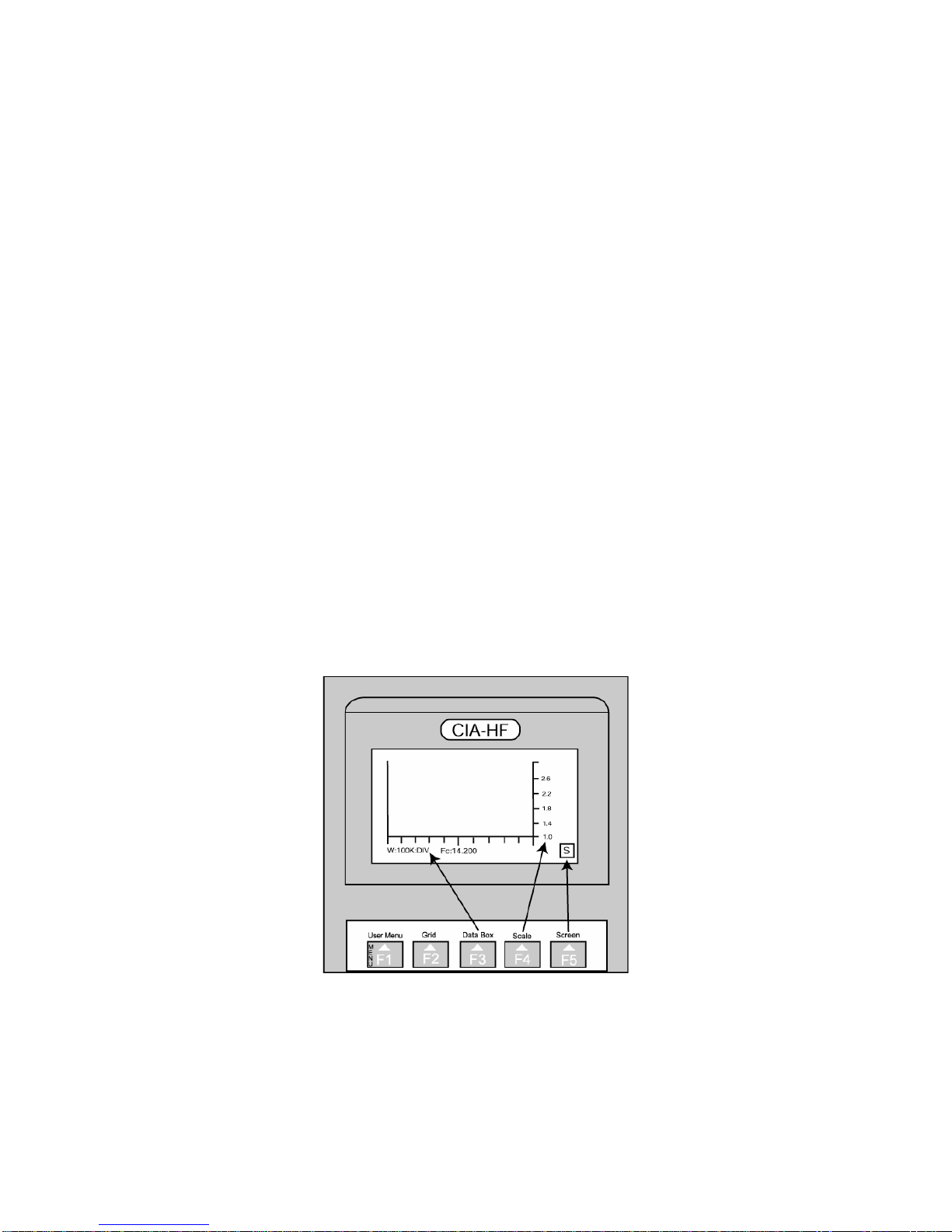
The five real time graphing screens include: SWR screen, Magnitude of Impedance screen,
Reactance screen, Resistance screen, and Vector screen. These screens contain a graphing
area, Data Box, and Logo Box (Figure1).
The graphing area is 100 pixels wide. It is bordered on the right by a vertical axis containing a
user-selectable scale, and on the bottom by a horizontal axis containing tick marks every ten
pixels. The center (longest) tick mark represents the center frequency (center of the plot).
The Data Box, which contains three (simple mode) to 12 (expert mode) data blocks, is located
below the horizontal frequency axis. The data blocks are updated after each frequency sweep,
center frequency adjustment, or width adjustment.
NOTE: A data block will display the acronym “NA” when numerical data is Not Available for a
particular value. This usually occurs when the SWR is too high or the Magnitude of Impedance is
too far from 50 ohms.
The Logo Box, located in the lower right hand corner of the display, contains a letter that identifies
the screen you are currently viewing. This box becomes vital in the expert mode when keeping
track of your location becomes a little more challenging. The following key lists the real time
screens and their identifying letters.
S………… SWR screen
Z………… Magnitude of Impedance screen (absolute value)
X………… Reactance screen (absolute value)
R………... Resistance screen (Real value of Impedance)
V………… Vector screen (rectangular display of Impedance, X vs. R)
D………... Data screen
N………… Numerical Entry screen (displays numbers entered on the keypad)
DEDICATED KEYS
The dedicated keys, which include all but the F1-F5 softkeys, are used to adjust operational
parameters.
The ON and OFF keys activate and deactivate, respectively, the Analyzer.
In the real time graphing screens, the WIDTH keys determine the frequency sweep range
represented in a plot (refer to Frequency Sweep Range section). To adjust this range, use the
WIDTHpand WIDTHqkeys to step through eight preset width values (0kHz, 10 kHz, 20 kHz, 50
kHz, 100 kHz, 200 kHz, 500 kHz, 1 MHz).
When the width is set to 0 kHz, the unit will analyze SWR, Impedance, etc. at a single frequency
(center frequency value). In addition, a beep sound at a rate that is proportional to the SWR at the
center frequency (i.e. a low beep rate indicates a low SWR). This auditory cue allows you to
make antenna adjustments without having to visually consult the display.
The center frequency of a plot, which defines the midpoint of the frequency sweep range, can be
adjusted in three ways. One way is to use the FREQpand FREQqkeys to step the center
frequency value up and down in increments one-tenth the width value. For example, when the
width is set to 500 kHz, the step size value will equal 50 kHz. Each time you adjust the width, the
step size value will also change. This automatic feature enables fine-tuning within a plot.
You can also use the number keys to enter new center frequency values. Simply input a value
between 0.001 and 54.000 MHz, followed by the ENTER key. Since the decimal point is in a fixed
position, zeros will precede any values that are less than five digits long (i.e. 00.545).

6
As soon as you begin inputting numbers, the Numerical Entry screen will appear (refer to screens
section). Once you press ENTER to terminate an entry, the Analyzer will resume normal
operation according to the new center frequency value.
It is also possible to use the number keys in conjunction with the FREQ keys to add or subtract
values from the current center frequency value. For example, entering 5 0 0 FREQpwill add 500
kHz to the current center frequency value. (The FREQqkey subtracts the input value from the
center frequency.)
In the user Menu (described below), the WIDTH and FREQ keys perform different functions. The
WIDTHpand WIDTHqkeys allow you to scroll through the user Menu selections. The FREQp
and FREQqkeys allow you to adjust the CONTRAST level and SWR Bandwidth values once
you have scrolled to these selections.
The ENTER key has multiple functions. In the Numerical Entry screen, it is used to terminate new
center frequency values entered on the keypad. In the real time graphing screens, pressing the
ENTER key reverses the direction in which the F3-F5 softkeys scroll through data, scale values,
and screens, respectively. A small minus (-) sign will appear in the Logo Box when the Analyzer
is in the reverse scrolling mode. Press the ENTER key again to revert to forward scrolling. Once
you become familiar with the sequence of data, scale values, and screens, you may find that
backward scrolling is more efficient than forward scrolling.
Pressing the EXAM/PLOT key in any of the real time graphing screens allows you to freeze the
display when you want to more closely examine a plot. In this EXAM mode, only the width and
center frequency values are accessible in the Data Box. In addition, the words “EXAMINE PLOT”
are displayed in place of the Logo Box. You cannot access any more data or make any plot
changes in this mode. Once you have finished examining a plot, press EXAM/PLOT again to
resume normal operation.
NOTE: In the EXAM mode, power is removed from much of the Analyzer’s circuitry. Enter this
mode whenever possible to extend battery life.
FUNCTION KEYS
The F1-F5 softkeys allow you to access different screens, data, and plot parameters.
F1: User Menu
Use the F1 softkey to toggle between the real time screens and the user Menu screen. This
screen contains a list of operational selections as well as a brief definition of each softkey. These
definitions are located in boxes directly above their corresponding softkeys.
The list of operational selections includes: TEST, KEYS, CONTRAST, SWR BW1, SWR BW2,
METER, and EXTRA FEATURES. A flashing arrow cursor is automatically positioned next to the
TEST selection whenever you enter this screen. Use the WIDTHpand WIDTHqkeys to cursor
through the list.
When the cursor is aligned with the TEST option, press ENTER to initiate a series of self-
diagnostic tests. The word “TESTING” will flash on the TEST line until the self-diagnostics are
complete, whereupon one of the three types of messages will appear. If the self-diagnostics do
not detect any problems, the “PASSED” message will appear. If the Analyzer detects low battery
levels, the “LO BAT” massage will appear –refer to the Internal Access section for battery
replacement information. Finally, if any problems are detected during the self-diagnostics, a
“FAILURE” message will appear. In this case, call AEA’s technical support department for
troubleshooting assistance (refer to In Case of Trouble section).

7
When the cursor is aligned with the KEYS option, press ENTER to display a new screen listing
the function definitions of the number keys and softkeys. Press ENTER a third time to return to
the main user Menu screen.
When the cursor is aligned with the CONTRAST option, use the FREQpand FREQqto adjust
the display contrast level.
The two SWR lines allow you to input specific SWR values (between 1.2 and 3.5) at which the
Analyzer will display the corresponding bandwidths. When the cursor is aligned with either SWR
selection, use the FREQ keys to adjust the displayed value.
Default values: 1.5 and 3.0
When the cursor is aligned with the METER option, press ENTER to display the Analyzer’s
remaining battery voltage. The Analyzer will also measure and display the Dc voltage of an
external voltage source connected to the antenna connector.
When the cursor is aligned with the EXTRA FEATURES option, use the ENTER key to toggle this
option ON and OFF. Turn this feature ON to activate the expert mode, which provides nine
additional data blocks and four additional real time screens.
Default: Off
F2: Grid
While viewing the S, Z, R, or X real time screens, press the F2 softkey to superimpose a grid
(graticule) over the plot. The grid allows you to more precisely determine values within a plot.
Press F2 again to remove the grid.
Default: Off
F3: Data Box
Use the F3 softkey to scroll through the data blocks located in the Data Box. This key is useful
because it allows you to access data without having to exit the real time screen. The three data
blocks that are available in both the simple and expert modes include:
W:xxx Fc:xxx Width, Center Frequency
SWR:xxx RL:xxx Standing Wave Ratio, Return Loss
Z:xxx R:xxx X:xxx <:xxx
Absolute value, Real component, Reactive component, and
Phase Angle of Impedance
To expand the number of data blocks displayed in the Data Box, enable the expert mode (refer to
the F1: User Menu section). In the expert mode, the following nine data blocks will become
available within the Data Box:
L:xxx C:xxx Inductance or Capacitance value relating to the Reactance at
the center frequency; describes the complex conjugate value
of the Inductance or Capacitance needed to resonate a load
to the center frequency
BW2.0:xxx Q:xxx 2:1 SWR Bandwidth in MHz, Q factor (Fc/2:1BW)

8
FL:xxx BW2.0: FH:xxx Lower Frequency @ SWR 2:1, Higher Frequency @ SWR 2:1
FL:xxx BW3.0: FH:xxx Lower Frequency @ SWR 3:1, Higher Frequency @ SWR 3:1
FL:xxx BW1.5: FH:xxx Lower Frequency @ SWR 1.5:1, Higher Frequency @ SWR 1.5:1
MIN SWR:xxx at F:xxx Lowest SWR, Frequency at which MIN SWR appears
NORMALIZED Z:xxx 50-ohm Normalized value of Z expressed as real ±j
Imaginary components
<xxx Fc:xxx xxx> Minimum, Center Frequency, maximum values in the frequency
sweep range
-xxx Fc:xxx +xxx Lowest frequency in the sweep range (Fc -half width), Center
frequency, Highest frequency in sweep range (Fc + half width)
F4: Scale
To change the vertical axis’ scale factor in the S, Z, X, and R screens, use the F4 softkey to scroll
through three sets of scale values. Use this feature to zoom in and out of a plot quickly.
Default values: 1.0-6.0
F5: Screen
Use the F5 softkey to scroll through the real time screens. Notice that the Logo Box will update as
you scroll through the screens.
Default: S screen
FREQUENCY SWEEP RANGE
During normal operation, the Analyzer continuously sweeps and plots a user-selected frequency
range. This range, termed the frequency sweep range, is defined by the width and center
frequency values.
Each tick mark on the horizontal axis represents an interval equal to the width value. When the
width is set to 100 kHz, for example, each tick mark represents an interval of 100 kHz. Thus, the
total frequency sweep range represented within the plot is 1000 kHz, or the sum of all ten
intervals. This can be simplified as Frequency Sweep Range = 10 x Width. The center frequency
value determines the midpoint of this 1000 kHz frequency sweep range.
With the EXTRA FEATURES function enabled, the Data Box displays the frequency sweep range
in three ways. For example, assuming the center frequency is set to 7.100 MHz and the width is
set to 100 kHz, the sweep range will alternately appear as “W:100K:DIV Fc:7.100”, which
indicates the basic plot values and lets you calculate the actual range, “<6.600 Fc:7.100 7.600>”,
which calculates the minimum, canter, and maximum frequency values represented in the plot,
and “-0.500 Fc:7.100 +0.500”, which simply informs you that the Analyzer is sweeping 500 kHz
above and below the center frequency value.

9
RESETTING THE INSTRUMENT
In the expert mode, the current screen and plot settings (i.e. center frequency, frequency step
size, scale value, and width) are saved when you turn off the Analyzer. This feature allows you to
power backup to the same screen and settings. To reset the Analyzer to its factory default
settings, press any of the number keys to enter the Numerical Entry screen. Then simply power
the Analyzer off. The next time you activate the Analyzer, it will operate according to the factory
default settings: center frequency: 14.200 MHz, width: 100 kHz, frequency step size: 10 kHz, and
scale: 1.0-6.0.
AUTOMATIC OFF
The Analyzer is programmed to automatically power off after a five minute idle period in order to
conserve battery power. The Analyzer begins to calculate the idle period each time you press a
key.

10
SECTION 4.
APPLICATIONS
The following examples by no means describe the extent of the Analyzer’s capabilities, but are
intended as jumping off points. To follow along with the examples, first activate the Analyzer’s
expert mode (refer to Function Keys section).
TUNING SIMPLE ANTENNAS
Example: Tuning an 80-meter inverted “V” antenna to 3800 kHz.
Process:
1. Insert the feedline of the 80-meter inverted “V” antenna into the Analyzer’s antenna
connector.
2. Turn the Analyzer on. When the S screen appears, press 3 8 0 0 ENTER to change the
default center frequency value to 3800 kHz. Maintain the default width value.
3. A “V” or “U”-shaped SWR curve will appear.
4. Using the F4 (zoom factor) softkey, select the lowest scale values that maintain the bottom of
the SWR curve below the scale’s midpoint. (You may have to experiment a little to determine
which scale values work.)
5. Determine on which side of the center frequency the bottom of the SWR curve rests. The
bottom of the curve should indicate the antenna’s resonant frequency.
6. To confirm the value of the resonant frequency, press F3 to scroll through the data blocks
until “MIN SWR:xxx at F:xxx” is displayed. This data block indicates the location of the
minimum SWR.
7. Press F5 to enter the Z screen. A “V” or “U”-shaped curve will appear, indicating the absolute
value of Impedance versus frequency.
8. Press F5 again to enter the X screen. The Reactance plot will dip down toward 0 ohms (on
the vertical scale) at the resonant frequency.
If the resonant frequency is higher than the center frequency in the SWR plot, you can assume
the Reactance is Capacitive. To tune the antenna to resonance, you either need to add equal
lengths of wire to each side of the “V” antenna, or add an inductor, in series with the center
conductor of the antenna’s feedline, at the feedpoint. Press F3 until the Data Box displays the
“L:xxx C:xxx” data block. The C:” value indicates the antenna’s equivalent series Capacitance at
the center frequency. The L:” value indicates the series Inductance (conjugate value) needed to
resonate the antenna at the center frequency. You will likely have to experiment with the
Inductance value to find an exact match. Depending on both the Impedance mismatch at the
antenna feedpoint and the length of the feedline, you can use either an inductor or capacitor, in
series with the center conductor of the feedline, to tune for resonance.
If the resonant frequency is below the center frequency, you can assume that the Reactance is
Inductive (i.e. the antenna is TOO LONG). In this case, perform the reverse of the operation
described in the above paragraph.

11
TUNING ½ AND ¼ TRANSMISSION LINES AND STUBS
Example: Using a standard Wilkenson power divider to stack two 15-meter yagi antennas with
two ¾ wave sections of RG-11, 75-ohm coax lines. The ¾ wavelength cable is used in this
example because two ¼ wavelength cables would not be long enough to allow optimum stacking
distance between the two antennas.
Process:
1. Use the following equation to determine the length of coax cable needed for ¼ wave phasing
lines. (For solid polyethylene coax, assume a velocity factor of 0.6.)
234 x Vf = 234 x 0.6 = 6.61 feet
F 21.250
For ¾ wave phasing lines, plug 6.61 feet into this equation:
6.61 x3 = 19.8 = 19 feet 9 5/8 inches
2. Cut two, 22 foot-long lengths of coax cable (the lengths of coax cable are cut approximately
10% longer than the computed length to allow for fine tuning).
3. Solder a coax “PL-259” connector to one end of each cable.
4. Attach the “PL-259” connector to a “T” connector already attached to the antenna connector.
Attach a 50-ohm load to the other end of the “T” connector (Figure 2).
5. Turn the Analyzer on. At this point, follow the steps for either the ½ Wave Cutting Method or
the ¼ Wave Shorting Method
FIGURE 2. T Connector
½ Wave Cutting Method
1. When the S screen appears, press the WIDTHpkey twice to select an initial width of 500
kHz. Enter 4 2 5 0 0 ENTER to set the center frequency to 42.500 MHz (the frequency at
which the tuned phasing lines will be 1.5 wavelengths). This center frequency value is twice
the 21.250 frequency value used in the above equation.
2. A “V” or “U”-shaped SWR curve will appear.
3. If the calculations for determining the length of the coax cable were correct, the SWR curve
should dip at a frequency of approximately 38.250 MHz. You are now ready to start tuning
the phasing line.

12
4. Begin cutting inch-long pieces off of the unterminated end of the phasing line. The resonant
frequency of the SWR curve will increase as the line is shortened.
5. As the SWR dip descends lower in the plot, shorten the cuts to ¼ inch long. This allows you
to finely tune the line. In addition, use the WIDTHqkey to increase the display resolution.
Use the F4 softkey to zoom in on the dip. Once the SWR reaches a minimum, your antenna
is tuned.
6. Repeat this process for the second phasing line. It is imperative that the bottoms of the two
SWR curves are aligned on the same frequency. If the bottom of one of the curves is at 0
over a narrow group of frequencies, average the two extreme frequencies where the SWR is
at a minimum.
¼ Wave Shorting Method
1. Enter 2 1 2 5 0 ENTER to set the center frequency to 21.250 MHz.
2. Use a very sharp ice pick to short through the coax cable.
3. Determine the position that produces the lowest SWR point at the center frequency. Cut the
cable at this point and install a coax connector. Your cable is now tuned.
4. Repeat this process for the second phasing line.
You can also use the ½ Wave Cutting or ¼ Wave Shorting methods described above to tune
phasing lines any number of degrees for a particular frequency. For example, if you want to cut a
transmission line for 21°at 3.795 kHz, simply use the following equation to determine the
frequency for 180°:
180 x 3.795 = 32.529 MHz
21
Since 21°at 3.795 kHz is equivalent to 180°at 32.529 MHz, simply use the ½ Wave Cutting
Method to tune the line for 32.529 MHz.
MEASURING INDUCTORS AND CAPACITORS
When measuring inductors and capacitors, it is highly recommended that you assemble an
accessory connector to maximize Analyzer accuracy. To do this, solder one end of a 50-ohm
resistor onto the center pin of a coax PL-259 connector. Then, splice an alligator test lead to the
resistor; solder a second test lead to the connector shell (Figure 3).
FIGURE 3. 50 OHM ACCESSORY CONNECTOR
For best results, when determining the value of an inductor or capacitor, take measurements at
the frequency where the Reactance of the load is equal to the 50-ohm resistor in the accessory
connector.

13
Inductors
Example: Determining the Inductance of a relatively small coil.
Process:
1. Plug the 50-ohm accessory connector into the Analyzer and clip the coil between the two test
leads.
2. Turn the Analyzer on and use the F5 softkey to scroll to the X screen. Enter 2 5 0 0 0 ENTER
to select an initial center frequency of 25 MHz. Press the WIDTHpkey until the width is set
to 1 MHz. Also, use the F4 softkey to set the scale to the 0-250 ohms range.
3. Unless you select a higher frequency, low Reactance will probably cause the plot to flat line
near the bottom of the screen. If Inductance is relatively high in higher frequencies, the
Reactance plot will flat line near the top of the scale.
4. Experiment with different center frequency values until you find the point at which the
Reactance plot reaches approximately 50 ohms.
5. Use the F5 to scroll the Data screen. The Phase Angle (<:) should read approximately 45°. If
it does not, press the FREQpor FREQqkey until it does. Now, identify the Inductance (L:)
value within the Data screen.
Capacitors
Example: Determining the Capacitance of a small capacitor (approximately 1000 pF).
Process:
1. Plug the 50-ohm accessory connector into the Analyzer, and clip the capacitor between the
two test leads.
2. Turn the Analyzer on, and use the F5 softkey to scroll to the X screen. Enter 5 0 0 0 ENTER
to select an initial center frequency of 5 MHz. Press the WIDTHpuntil the width is set to 1
MHz.
3. The Reactance plot will sweep down from the left side of the display, leveling out as it
approaches the right side.
4. Adjust the center frequency value until you determine the point at which the Reactance is
approximately 50 ohms.
5. Press F3 until the “Z:xxx X:xxx R:xxx <:xxx” data block is displayed. The Phase Angle (<:)
should read approximately 45°since the R and X values are roughly equal. If it does not,
adjust the center frequency until it reads as close to 45°as possible.
6. Press F3 to scroll to the “L:xxx C:xxx” data block. Refer to the “C:” value to determine
Capacitance.
TUNING ANTENNA TRAPS
Example: Using the 50-ohm accessory connector constructed for the above example to tune an
antenna trap (composed of a coil in parallel with a capacitor).
Process:
1. Leave the coil and capacitor of the trap connected at one end, separated at the other.
2. Clip one test lead of the accessory connector to the coil, the other test lead to the capacitor.
3. Turn the Analyzer on. Maintain the default S screen and plot values.
4. Determine on which side of the center frequency the bottom of the SWR curve rests. The
bottom of the curve should indicate the antenna’s resonant frequency.
5. To confirm the value of the resonant frequency, use F3 to scroll through the data blocks until
“MIN SWR:xxx at F:xxx” is displayed. This data block indicates the location of the minimum
SWR.
6. Press F5 to enter the Z screen. A “V” or “U”-shaped curve will appear, indicating the absolute
value if Impedance versus frequency.
7. Press F5 again to enter the X screen. The Reactance plot will dip down toward 0 ohms (on
the vertical scale) at the resonant frequency.
8. Refer to the analysis paragraphs following the “Tuning a Simple Antenna” procedure.

14
DETERMINING RESONANT FREQUENCY
Example: Using the 50-ohm accessory connector constructed for the above example to
determine the resonant frequency of an LC-tuned circuit.
Process:
1. Use the test leads of the 50-ohm accessory connector to connect the inductor and capacitor
in series.
2. Turn the Analyzer on. Maintain the default S screen.
3. Find the resonance point of the circuit by locating the lowest SWR point.
4. Use the FREQ keys to center the lowest SWR point.
5. Access the Data screen to read the 2:1 SWR bandwidth and the Q factor directly.
DETERMINING CHARACTERISTIC IMPEDANCE
For this type of measurement, you will need to assemble another accessory connector using a
500-ohm potentiometer (Figure 4).
FIGURE 4. 500 OHM POTENTIOMETER CONNECTOR
Example: Determining the characteristic Impedance of an unknown coax cable.
Process:
1. Attach the unknown cable to the Analyzer’s antenna connector. Attach the potentiometer
accessory connector to the unterminated end of the cable using a PL-258 barrel connector.
2. Use the F5 softkey to scroll to the R screen. Press 2 5 0 0 0 ENTER to select a new center
frequency value of 25 MHz, and press the WIDTHpkey until the width is set to 1 MHz. Use
the F4 softkey to set the vertical scale to 100 ohms full scale.
3. Depending on the length of the cable (hopefully at least 25 feet), two or more sine waves will
appear on the display.
4. Use the potentiometer to adjust the plot for minimum amplitude variance on the sine waves.
5. Now, disconnect the potentiometer from the cable. Use a volt-ohmmeter to determinethe
Resistance of the potentiometer. Usually a 50-ohm cable will read between 49 and 52 ohms
of Resistance. It is also possible to read the Resistance value of the potentiometer by
disconnecting it from the cable and plugging it directly into the Analyzer. Use the F5 softkey
to scroll to the Data screen; once there, identify the Resistance (R:) value.
TESTING BALUNS
Example: Using the 500-ohm potentiometer accessory connector constructed for the above
example to determine the output (or input) Impedance of an unknown balun.
Process:
1. Insert the 50-ohm port of the balun into the Analyzer, and the potentiometer connector into
the balun’s vacant port.
2. Turn the Analyzer on. Maintain the default S screen.
3. Adjust the potentiometer for minimum SWR. (The balun may not flat line over a wide range of
frequencies.)
4. To identify the balun’s useful range, experiment with different center frequency and width
values. You may see larger SWR values at the extreme lower and upper frequencies.
5. To determine the balun’s Resistance, disconnect the potentiometer from the balun and plug it
directly into the Analyzer. Then, access the Data screen (F5 softkey) to identify the
Resistance (R:) reading.

15
ADJUSTING ANTENNA TUNERS
Example: Adjusting an antenna tuner without transmitting a signal on the air.
Process:
1. Connect a cable from the input of your antenna tuner to the center connector of a two-
position coax switch (be sure to use a switch that shorts the unused portion).
2. Connect the open position of the switch to the output of your transceiver.
3. Connect a cable from the closed position of the switch to the antenna connector on the
Analyzer.
4. Turn the Analyzer on. Set the center frequency and width values of your choice. Use the F5
softkey to scroll to the Z screen.
5. Adjust the tuning on the antenna tuner (with the proper antenna connected to the antenna
tuner output) until the center frequency displays an Impedance value of 50 ohms.
6. Use the F5 softkey to scroll to the X screen to make sure Reactance is zero.
7. Use F5 to scroll to the S screen. Note the low SWR value at the center frequency. Flip the
coax switch to the transceiver. The low SWR presented to the Analyzer will now be presented
to the transceiver.
MEASURING CABLE LENGTH/DISTANCE TO FAULT
NOTE: The following data block will be referenced in this addendum:
“Fc:xxx VF:xxx FT:xxx (x)” Center Frequency, Velocity Factor, Feet, (O) Open or (S) Short
The Analyzer measures the physical length of a coax cable, or the distance to the first short or
open present on a coax cable, by determining the frequency at which cable impedance goes to
zero. This frequency is inversely proportional to the length of the cable, and is used, along with
the user-programmable velocity factor, to compute the distance to the end of the cable.
Generally, an open cable will exhibit a nearly zero impedance at the ¼ wavelength frequency.
Example: Determining cable length/the distance to an open or short present on a coax cable.
Process:
1. Attach the coax cable under test to the antenna connector. Turn the Analyzer on.
2. Press F1 to access the user Menu screen. Use the WIDTHqkey to scroll down to the “VF:50
(open)” (velocity factor) selection
3. Use the FREQpand FREQqkeys to change the velocity factor to a value between 0.50 and
0.99. (The velocity factor for your cable is listed in the Radio Amateur’s Handbook or in the
ARRL Antenna Handbook, or is available directly from the manufacturer.) If you toggle past
0.99, the velocity factor value will revert to 0.50, and the fault type indicated in parentheses
will change from OPEN to SHORT and vice versa. NOTE: A correct velocity factor is critical
in obtaining accurate distance measurements.
4. Press F1 to return to the real time graphing screen. Use F3 to scroll to the “W:xxx Fc:xxx”
data block. Input 5 0 0 0 ENTER to set the center frequency to 5.000 MHz. Use the WIDTHp
key to set the width to 1 MHz.
5. Use F5 to scroll to the Z (impedance) screen.
6. Depending on the length of the cable, you should observe one or several dips in the
impedance curve. Select the LOWEST center frequency value (above zero) that displays a
full dip. Experiment with the center frequency value until it is as close to the center of the dip
as possible. As a general rule, enter lower center frequencies for longer cables and higher
center frequencies for shorter cables. For example, enter a center frequency of 5.000 MHz to
display the dip of a 32-foot long cable possessing a velocity factor of 0.66.
7. Press ENTER to reverse data block scrolling. Press F3 once to display the “Fc:xxx VF:xxx
FT:xxx (x)” data block. Consult the “FT:” reading to determine the length of the cable. If the
footage reading is shorter than expected, an open or short may be present on the cable at
the distance indicated.

16
If there is a known fault on the cable, and the distance to fault (“FT:”) reading seems inaccurate,
verify that the open termination is truly an infinite DC open, or that the short is a direct short with
no inductance. An incorrect velocity factor will also contribute to an inaccurate footage reading.
Occasionally, a cable’s true velocity factor will vary from the published or manufacturer
specification because of a production variance or because of cable deterioration due to ultraviolet
or water contamination. Please note that since the velocity factor is allotted only two decimal
places, it is not possible to measure distance with better than 1% accuracy.
MEASURING CABLE LOSS
Example: Determining cable loss.
Process:
1. Turn the Analyzer on.
2. Before you attach the cable under test, enter the center frequency at which you want to
determine Return Loss.
3. Use F3 to scroll to the “SWR:xxx RL:xxx” data block. The “RL:” reading should be less than 2
dB, depending on the center frequency selected. Note this reading.
4. Now attach the cable under test to the antenna connector. Note the new Return Loss
reading. Confirm that the cable under test has either a direct short or a complete open at the
termination end.
5. Subtract the initial Return Loss reading (without the cable connected) from the new reading.
The result is the total (round-trip) Return Loss present in the cable.
6. Divide the result by two (2) to determine actual cable loss (one-way) at the selected center
frequency.
OTHER APPLICATIONS
Uses for the CIA-HF Analyzer are limited only by your imagination and experience. We
encourage you to explore all of the Analyzer’s capabilities –those listed here and those wanting
to be discovered. For more information on Antenna Impedance Matching, consult the ARRL
Antenna Handbook.

17
REMOTE OPERATION
SERIAL PORT PROTOCOL
9600 baud
8 data bits
no parity
1 stop bit
POWER UP
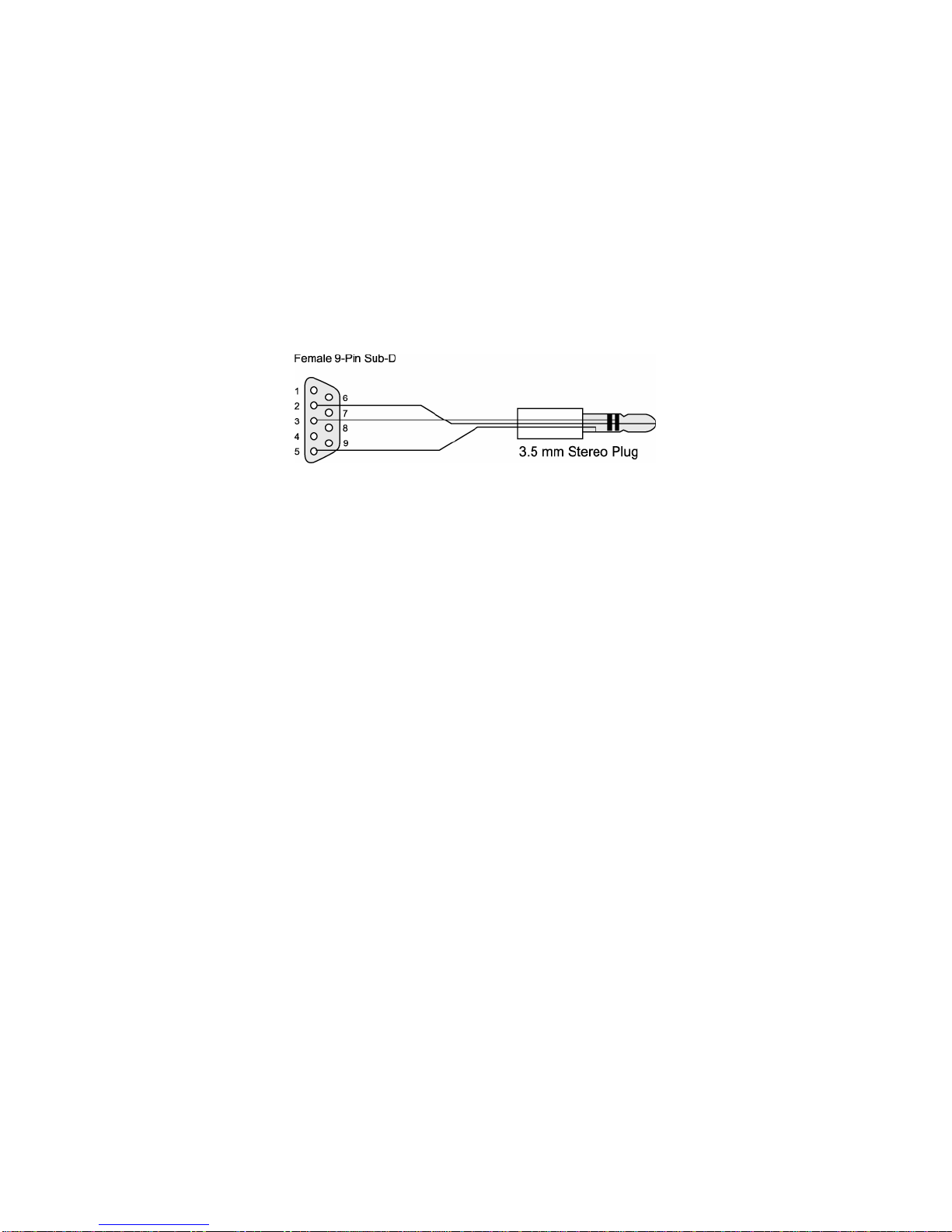
To perform remote operation, you will need to connect the Analyzer to your PC via a serial
interface cable. You have the option to assemble a cable yourself or purchase one of the serial
interface cables, displayed below, directly from AEA.
The Analyzer can be powered up manually, using the ON key, or remotely, using your PC. To
remotely power up the Analyzer, simply send the letter “K” until you receive a “?” in response. At
this point, you can begin sending commands. When the Analyzer is already powered on, it will
automatically time out after a five-minute idle period in order to conserve batteries. It will power
back up when it detects an incoming serial stream.
RULES FOR COMMANDS
uAll commands must be in upper case letters. Lower case letters are invalid
uAll incoming commands to the Analyzer must be terminated with the letter “K”. If the Analyzer
detects an incoming stream containing ten or more characters, that is not terminated with the
letter “K”, it will output a “?” and discard the characters. (All commands contain fewer than ten
characters.)
uAll outgoing responses from the Analyzer are terminated with either a “K” or a “?”. The letter
“K” indicates that the incoming command was properly executed and that no further
information is outgoing. The “?” indicates that the Analyzer did not understand the incoming
command. Re-enter the proper command.
uThe analyzer will accept commands manually entered on its keypad or remotely transmitted
from a terminal (serial commands). Do not attempt to use both methods at the same time. The
Analyzer will not accurately respond to mixed manual and serial commands.
COMMANDS
The following serial commands direct the Analyzer to perform certain functions. Remember, each
of these commands must be terminated with a “K” (as shown).
SK Send 100 SWR data points
ZK Send 100 Z (Impedance Magnitude) data points
XK Send 100 X (Reactance) data points
RK Send 100 R (Resistance) data points