Eosense eosFD User manual

User Manual
eosFD
eosFD Forced Diffusion
Chamber and Software

User Manual
This guide is distributed by EOSENSE INC (“Eosense'') for users of the eosFD Forced Diffusion
chamber instruments in conjunction with the eosLink-FD software. Eosense is not liable for special,
indirect, incidental, or consequential damages. Eosense's obligation under this warranty is limited to
repairing or replacing (at Eosense's discretion) defective products within one (1) year from date of
delivery to the customer. The customer shall assume all costs of removing, reinstalling, and shipping
defective products to Eosense where applicable. Eosense will return said products by surface carrier
prepaid. This warranty is in lieu of all other warranties, expressed or implied.
This product complies with the following directives for CE Marking:
2011/65/EU (RoHS2)
2015/863/EU (RoHS3)
2004/108/EC (Electromagnetic compatibility)
For more information, contact [email protected]
Version: 3.1
Revised: August 2020
1 [email protected]
© Eosense Inc.

User Manual
Contents
Contents 2
1 Summary 3
2 Introduction 4
2.1 What is Forced Diffusion? 4
2.2 How is Flux Calculated? 4
2.3 The Measurement Cycle 6
3 Quick Start Guide 7
4 Hardware 9
4.1 eosFD Housing 9
4.2 Main Power and Data Cable 9
4.3 Power Connectors 10
4.4 Data Cables 10
4.5 Analog Data 11
5 Deployment 12
5.1 Setup 12
5.2 Maintenance 13
6 Using eosLink-FD 14
6.1 Overview 14
6.2 Installing and Connecting 14
6.3 Using the eosLink-FD Interface 14
6.3.1 Menus 15
6.3.1 Buttons 20
6.3.1 Status Bar 23
7 Logged Data Files 24
8 Troubleshooting 25
2 [email protected]m
© Eosense Inc.

User Manual
1 Summary
This manual outlines the operation and features of the eosFD-CO2carbon dioxide (CO2) Forced
Diffusion (FD) chamber, as well as the included eosLink-FD software package. Before supplying power
to the eosFD, please ensure that you read the section on Power Connectors (4.3) to avoid any damage
to the sensor. We strongly recommended that all users read the complete manual before use.
This manual is intended for users of the eosFD with version 2.4.4 of the eosLink-FD interface. Please
check the Resources section of the Eosense website for the most up-to-date manuals and software.
If you have any specific questions or require additional guidance or information, please contact
Eosense Technical Support through our website, by phone or by email:
[email protected]
888.352.8313
https://eosense.com/contact-support/
➔Want to jump right into collecting flux measurements? Section 3 (Quick Start Guide) tells you
all you need to know to start out. For best results, we do recommend you read the entire
manual!
➔Want to learn more about customizing your eosFD measurements? Section 6 (Using
eosLink-FD) explains how to change the measurement frequency and collect data, as well as
other important instrument settings
➔Running into problems? Section 8 (Troubleshooting) covers some of the most common issues
and how to address them. And you can always contact us directly at [email protected].
➔Please visit the Resources section of our website at https://eosense.com/resources/ for
additional information and eosFD Application Notes, including:
◆AN0008: Sizing a Solar Power Supply for a Remote eosFD Installation
◆AN0012: eosFD Effects on Soil Moisture and Temperature
◆AN0014: Interfacing the eosFD to a Campbell Scientific CR1000/CR6 Data Logger
3 [email protected]m
© Eosense Inc.

User Manual
2 Introduction
2.1 What is Forced Diffusion?
The eosFD is a stand-alone soil CO2flux sensor, containing a single NDIR sensor, an internal data
logger and small diaphragm pump. The eosFD uses Eosense’s patented Forced Diffusion technology
to measure soil CO2flux directly. Traditionally, gas fluxes from the soil surface are measured using
closed chamber systems, with these “accumulation chambers” trapping gas during the measurement
period. CO2concentrations continue to increase while the chamber is down, and different mathematical
fits (typically linear or exponential) are applied to the data to indirectly estimate the original rate of flux.
Forced Diffusion is a membrane-based steady-state approach for measuring gas flux that establishes
an equilibrium between gas flowing into the chamber and gas flowing out of the chamber through the
membrane, without any external chamber movement. By carefully characterizing the diffusive
properties of the membrane used in the instruments, the eosFD chamber gas concentration can be
correlated directly to the gas flux rate. Essentially, the amount that this membrane limits the flow of gas
out of the chamber is known, and thus by comparing the internal concentration to that outside of the
instrument, the flux rate can be calculated. Unlike other automated chambers that lift and lower onto the
soil surface, the Forced Diffusion approach does not require external moving parts, allowing it to be
deployed in the harshest climates for extended periods without intervention.
2.2 How is Flux Calculated?
Forced diffusion flux is calculated by calibrating the diffusive transport of gas across the eosFD’s
membrane. This flux rate depends on the effective diffusivity of the interface, the concentrations on
either side and the path length between the two points. The relationships between these parameters
are linear, and everything but the soil and atmospheric concentrations are assumed to be constant,
which simplifies to a single calibration slope (G  ). The flux is then calculated by multiplying the difference
in soil and atmosphere concentrations by the calibration slope:
The full differential equation showing the (volume/surface area) scaled
rate of change in flux rate equal to the flux from the soil surface (F 
S 
)
minus the difference in concentration, ∆C (scaled by both the path
length L  and the diffusivity of the interface, D  ).
The change in the flux rate is assumed to be zero (steady-state) over
the timespan of the concentration measurements (~60 s). The
steady-state assumption reduces the equation to a linear dependence.
As the path length and interface (membrane) diffusivity are constant,
this can be represented by a single coefficient, G  .
4 [email protected]m
© Eosense Inc.

User Manual
In order to measure the difference in
concentration used to calculate flux,
the eosFD has two internal chambers
where gas is exchanged with the
atmosphere - the Soil Cavity and the
Atmospheric Cavity. Gases emitted
from the soil surface flow into the
bottom of the eosFD and accumulate in
the Soil Cavity. This gas is exchanged
with the atmosphere through two of the
membrane covered windows near the
bottom of the eosFD. The other two
windows lead to the Atmospheric
Cavity, which encircles the inner Soil
Cavity, but is isolated from direct
exposure to soil gas.
When the measurement cycle occurs,
samples from these two cavities are
drawn (via internal pump) to the NDIR
CO2sensor for analysis, before being
returned to the original cavity. These
measurements are used to calculate
the difference in concentration, ∆C.
For more information: Risk, D., Nickerson, N., Creelman, C., McArthur, G., Owens, J., 2011. Forced diffusion
soil flux: a new technique for continuous monitoring of soil gas efflux. Agric. For. Meteorol. 151, 1622–1631.
5 [email protected]m
© Eosense Inc.

User Manual
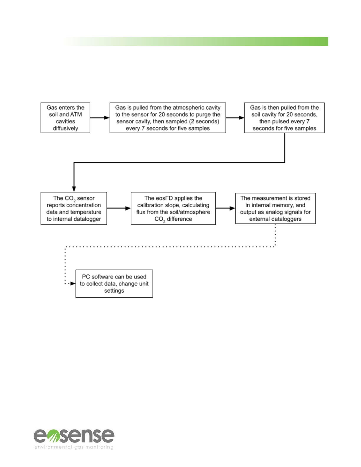
2.3 The Measurement Cycle
The eosFD samples gases from both the atmospheric and soil cavities within the device. The flow
diagram below breaks down the steps that the eosFD goes through to calculate flux.
When gas is being transported to and from the sensor cavity, the eosFD’s pump will be active, creating
a distinct buzzing sound. This sound is also emitted when the unit is turned on (three short pulses) or
when the eosFD accepts a command or data from the eosLink-FD software (one longer pulse).
Please note that how frequently the eosFD pump is active will depend on your measurement frequency.
For the default 10 minute setting, you will hear the eosFD alternate between long (~20 second) pump
activation and shorter (~2 second) pulses. This pattern will repeat twice per eosFD flux measurement,
with the length of silence between measurements depending on the measurement frequency setting.
6 [email protected]m
© Eosense Inc.

User Manual
3 Quick Start Guide
The following steps will guide you through the basic setup and use of an eosFD chamber, with detailed
information available in later sections of the manual.
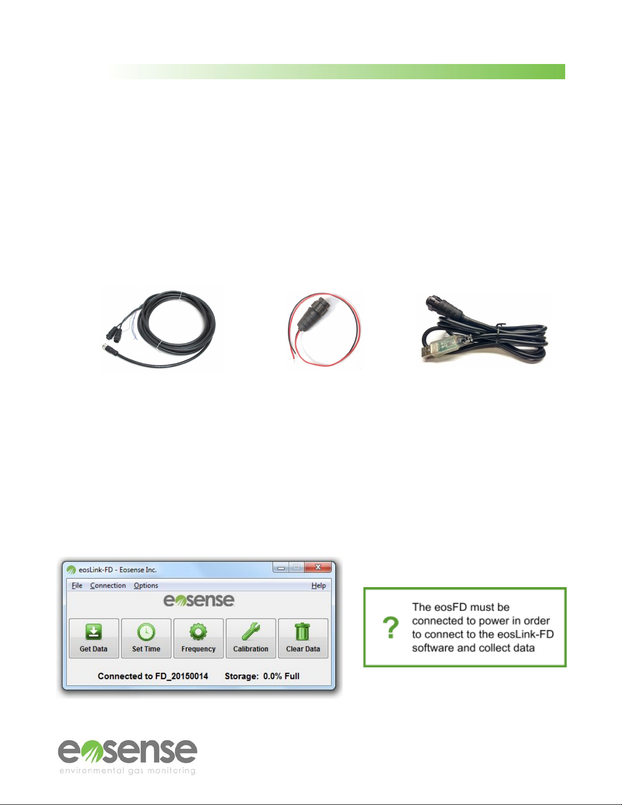
1.
●First connect the uncapped socket of the eosFD to the single, 12-pin end of the SSC
Power and Data cable.
●Connect the DC+ Power Cable to the 2-pin end of the SSC Power and Data Cable then
to a 12+ VDC power supply, with the red lead going to positive and the black going to
negative / ground (see Section 4.3: Power Connectors). The eosFD should pulse the
pump three times.
●Connect the 3-pin end of the SSC Power and Data Cable to the USB-RS232 Cable.
SSC Power and Data Cable DC+ Power Cable USB-RS232 cable
2. Connect to the device using a Windows based PC, the eosLink-FD software, and the included
data cable.
3. Check that the device’s system time is set appropriately, and choose a measurement frequency
(see Section 6: Using eosLink-FD). Exit the program and then disconnect the USB-R232 cable.
Sampling will begin automatically once disconnected from the eosLink-FD software if the eosFD
remains connected to power (when the first measurement begins will depend on the frequency
settings).
7 [email protected]m
© Eosense Inc.

User Manual
4. Attach the provided Mounting Ring to the top of the eosFD. Clear any vegetation from the soil
surface and gently insert the chamber into the soil surface (depth of approximately 1.5 cm) or a
previously installed collar, making sure that the bottom of the eosFD is flush with the soil surface
(see Section 5: Deployment). Use pegs and line to secure the eosFD to the soil surface via the
Mounting Ring.
5. If using an external data logger to record FD measurements, connect the purple wire for flux,
the blue wire for soil CO2concentrations, and/or the grey wire for temperature. Each wire
should be connected with one of the black grounding wires as a 0-5 VDC differential voltage
measurement (see Section 4.5: Analog Data).
6. After the desired monitoring time period has elapsed, connect to the device again as described
in Steps 2 and 3 above. Use the Get Data button to transfer the data file to your computer.
8 [email protected]m
© Eosense Inc.

User Manual
4 Hardware
4.1 eosFD Housing
The eosFD housing is machined from acetal plastic, allowing for a durable, water-resistant and
lightweight design. The instrument contains a single CO2sensor, an internal data logger and a small
diaphragm pump. The housing incorporates a diffusive membrane, electrical interface ports and
detachable leg mounting points for a stable field deployment.
The eosFD membrane is critical to proper operation of the device. The membrane should always
appear uniform in colour and free from visible defects. It is important to periodically check the
membrane, as use in field conditions may cause it to tear or otherwise become defective, and the
membrane will degrade naturally over time. Membranes should be replaced annually for best results,
though the membrane life-cycle may be shortened by exposure to harsh conditions. If dirty, membranes
can be cleaned using a gentle tool, such as a soft toothbrush, and a squirt bottle of deionized water.
Use the toothbrush lightly to dislodge any stubborn mud / sediment and then the squirt bottle to wash it
off. Avoid using any solvents such as alcohol, as this can damage the probe's water resistance
New eosFDs have one 12-pin socket. If using an eosFD with
two sockets (one capped and the other uncapped), be mindful
to use the uncapped socket when connecting the eosFD to
power and/or the computer. The capped socket is for
troubleshooting purposes only and should not be used.
4.2 Main Power and Data Cable
The eosFD ships with a standard 5 m power and data cable
(SSC), shown in Figure 1, which plugs directly into the uncapped
12-pin socket on the eosFD housing. Power is supplied to the
eosFD via the two pin connector on the opposite end of the SSC.
This connector also has a tab and notch type system to ensure
that the user connects power with the correct polarity. The eosFD
may be powered by supplying regulated 12 VDC to the sensor via
data logger, battery or other power supply device (see section 4.3:
Power Connectors). A longer 10 m cable (SLC) is also available.
Sensor data is stored on the internal data logger, which can be
accessed using the 3-pin data connector on the SSC, combined
with the USB-R232 cable. The eosLink-FD software is used to
collect stored data, as well as change any of the instruments
settings (see Section 6: Using eosLink-FD). Figure 1 SCC Power and Data cable
9 [email protected]m
© Eosense Inc.

User Manual
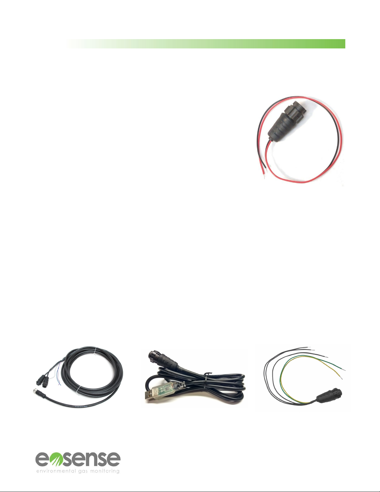
4.3 Power Connectors
The DC+ external power cable (Figure 2) included with the eosFD is
used to power the chamber from a DC power supply.
The DC+ cable includes a 2-pin connector for attachment to the
SSC/SLC cables. The opposite end of the cable has bare leads, to
allow for connection to a DC power supply. The black wire should be
attached to the ground terminal of the DC power device, and the red
wire should be attached to the positive terminal. The eosFD operates
on 12 V DC power. Exceeding 12 V may damage the eosFD, please
ensure that the voltage is regulated correctly before connecting the
power supply to the unit. The power consumption will vary slightly
depending upon the supplied voltage. The average draw for a 10
minute cycle is ∼100 mA (1.2 W) with a peak of ∼300 mA (3.6 W).
Figure 2 DC+ Power Cable
4.4 Data Cables
Communication between eosLink-FD and an eosFD uses the RS-232 Serial protocol. The following
components may be used to facilitate this interface:
● SSC Power and Data Cable - (Included) Used to power an eosFD as well as provide an RS-232
interface.
● USB-RS232 Cable- (Included) Connects the SSC data port to a USB port. Used to create a
virtual COM Port, allowing the eosFD to be connected to a computer through a USB port.
●Serial Breakout and Grounding Cable - (Included) Used to connect the eosFD to a data logger
using a serial interface. Also used as the grounding cable for analog connections (see section
4.5 for more information).
Figure 3 SSC Power and Data Cable (left), USB-RS232 Cable (middle), and
Serial Breakout and Grounding Cable (right)
10 [email protected]m
© Eosense Inc.

User Manual
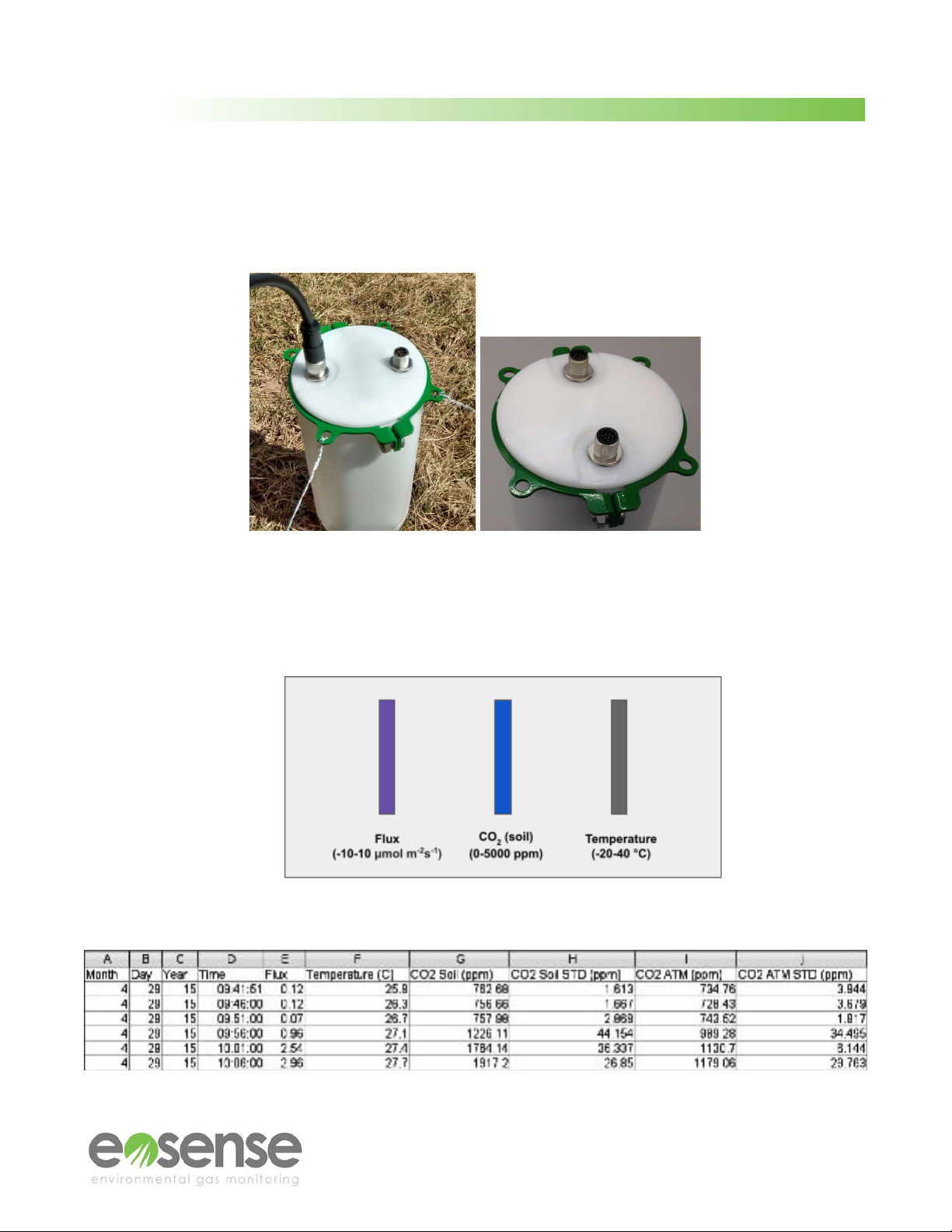
4.5 Analog Data
In addition to the internal memory of the eosFD, users also have the
option of recording analog data on an external data logger, using the
three wires on the SCC Power and Data Cable (AN0014 provides more
detailed information on interfacing an eosFD to a Campbell Scientific
data logger, including how to record data using the serial interface).
Each wire should be connected along with one of the three black
grounding wires as a 0-5 V DC differential voltage measurement, with
ranges, multipliers and offsets as shown in the table below:
Figure 4 Purple, blue, and grey
wires on the SSC Power and
Data Cable.
*New eosFDs no longer output Soil CO2via analog. CO2values recorded by the eosFD are used
only to calculate the flux, and are not intended to be stand-alone measurements of CO2.
In order to interpret the analog signals, simply apply the appropriate linear transformation to the voltage
data, as determined by the range. For example, to transform a temperature voltage signal, first divide
the voltage by the 0-5 V range, then multiply by the -20-40 °C temperature range. Finally, add the
minimum of the temperature range. The example below shows each step for a reading of 3 V.
(1) 3 V / (5 V - 0 V) = 0.6
(2) 0.6 * (40 °C - -20 °C) = 36 °C
(3) 36 °C + -20 °C = 16 °C
Thus a 3 V analog signal for temperature corresponds to 16 °C.
11 [email protected]m
© Eosense Inc.
Output
Colour
Units
Range
Multiplier
Offset
CO2 Flux
Purple
μmol/m2/s
-10 - 10
0.004
-10
Soil CO2 Signal*
Blue
ppm
0 - 5000
1.0
0
Sensor Temperature
Grey
°C
-20 - 40
0.012
-20

User Manual
5 Deployment
5.1 Setup
12 [email protected]m
© Eosense Inc.
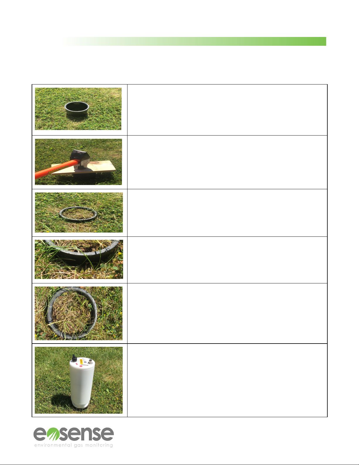
Situate the collar in a flat location, clear of any rocks or debris.
Remove any larger vegetation from the general area. When
possible, deploy the collar at least 24 hours prior to the start of
eosFD measurement collection (or allow for some disturbance
-related fluxes in the early portion of your data).
Gently tap the collar into the ground, ensuring that the force is
distributed evenly across the top of the collar. This can be
accomplished by placing a board or other flat object on top of the
collar, and using a broad-head hammer. Ensure that the top of the
collar remains parallel to the ground by tapping directly above the
collar and not to one side or the other.
Where possible, insert the collar to near full depth, as excessive
distance between the soil surface and the bottom of the eosFD can
increase how long it takes the instrument to respond to changing
flux rates. Ideally, a centimeter of space should be left, to aid in
installation of the eosFD itself as well as collar retrieval.
Inspection of the edges of the collar should show no significant gaps
between the soil and collar, though some near-surface spacing is
unavoidable. Upon subsequent visits to the field site, review these
edges, as the soil should naturally fill in any gaps created during
installation.
Try to minimize disturbance to the soil during collar installation, as
this can increase the equilibration time between the eosFD and the
soil, and potentially cause measurement errors if there is a
particularly bad seal between the soil and collar at depth.
To deploy the eosFD in the installed collar, simply insert one side of
the bottom ring into the collar until flush, then gently push on the
opposite side until the eosFD is securely seated. Inspect all sides to
ensure no gaps exist.

User Manual
While the eosFD is water resistant, avoid situating the probe in areas
of standing water or hollows where flooding is a possibility. For best
results choose a flat, clear soil surface that is free of large rocks to
insert the chamber. Where stability is a concern, use pegs and line to
secure the eosFD to the soil surface via the attached Mounting Ring,
ensuring that the guy-lines remain taut when the pegs are driven into
the soil.
Connect the eosFD to the 12-pin end of the SSC Power and Data
cable. Connect the DC+ Power Cable to the 2-pin end of the SSC
Power and Data Cable then to a 12 VDC power supply. Once
powered, the eosFD will pulse the pump 2-3 times, which indicates
that it is properly connected.
Figure 5 An eosFD deployed in
the field, with uncapped aux port
5.2 Maintenance
The eosFD should be checked-over monthly for best results. Check
the power supply and connection, ensuring that the eosFD pump
sounds when power is cycled. In the event of fouling, the eosFD
membrane can be cleaned by first gently removing any particles
using a dry, non-abrasive cloth. Then, use a damp (no solvents)
cloth to gently remove any remaining dirt or substance.
If the membrane appears to be significantly clogged or punctured
in any way, contact Eosense immediately to determine if the
membrane needs to be replaced. A damaged or fouled membrane
can lead to inaccurate flux measurements by the device. Make
sure to remove any vegetation growing in the collar or directly
around the eosFD that may block the side membrane. Finally,
ensure the collar is still flush with the surface, re-adjusting if
necessary. Figure 6
Top: Mildly fouled membrane.
Bottom: Clean eosFD membrane.
13 [email protected]m
© Eosense Inc.

User Manual
6 Using eosLink-FD
6.1 Overview
eosLink-FD is an application that allows the user to communicate with the eosFD chamber in order to
change various instrument settings, as well as collect and clear logged data. eosLink-FD is compatible
with Windows PCs.
6.2 Installing and Connecting
Simply copy the eosLink-FD.zip file (available on the Resources section of our website, or by contacting
us at: [email protected]) to a suitable directory on the PC in use, then unzip the file, which
contains the eosLink-FD software folder. None of the files in this
folder should be removed or changed in any way. If this occurs,
simply delete the entire folder from your PC and re-extract from
the zip file to re-create the folder.
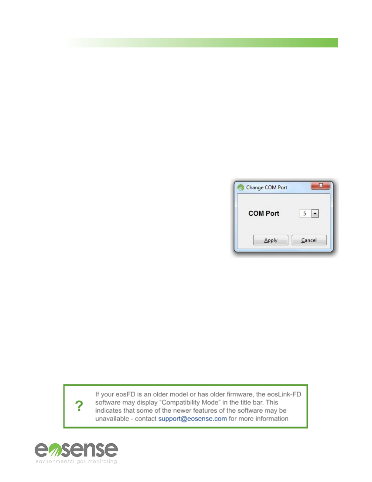
We recommended that you connect the data cable to your
computer prior to launching eosLink-FD; however you may also
refresh the program from the Connection menu. You may have
to refer to the Windows Device Manager if several serial port
devices are connected to the computer, and choose the correct
port through (Options⇒Change COM Port).
Figure 7 eosLink-FD Change COM Port
window
Once the port is selected, the eosFD will automatically attempt to connect. When the connection is
successfully established, the grayed out buttons and text will become active, and the eosFD serial
number and storage capacity will be shown at the bottom of the window.
6.3 Using the eosLink-FD Interface
The eosLink-FD window consists of four menus, five buttons and a status section at the bottom, as
detailed in the following subsections. Once the eosFD has been connected, the user can begin
modifying instrument settings. Left idle, the eosFD will automatically disconnect after ten minutes of
inactivity (timeout restarted every time a command is sent).
14 [email protected]m
© Eosense Inc.

User Manual
6.3.1 Menus
There are four menus visible at the top of the eosLink-FD window:
Menu 1 - File: This menu provides the ability to collect both the measurement data file and the error log
file (both commands also have their own dedicated button) as well as a means of exiting the program.
Menu 2 - Connection: The Connection menu has three options, including the ability to refresh the list
of available COM ports and choose a specific port number. If the program was launched prior to the
eosFD being connected, you will need to refresh the connection to allow the correct port to be chosen.
Menu 3 - Options: This contains a number of secondary functions which are described below.
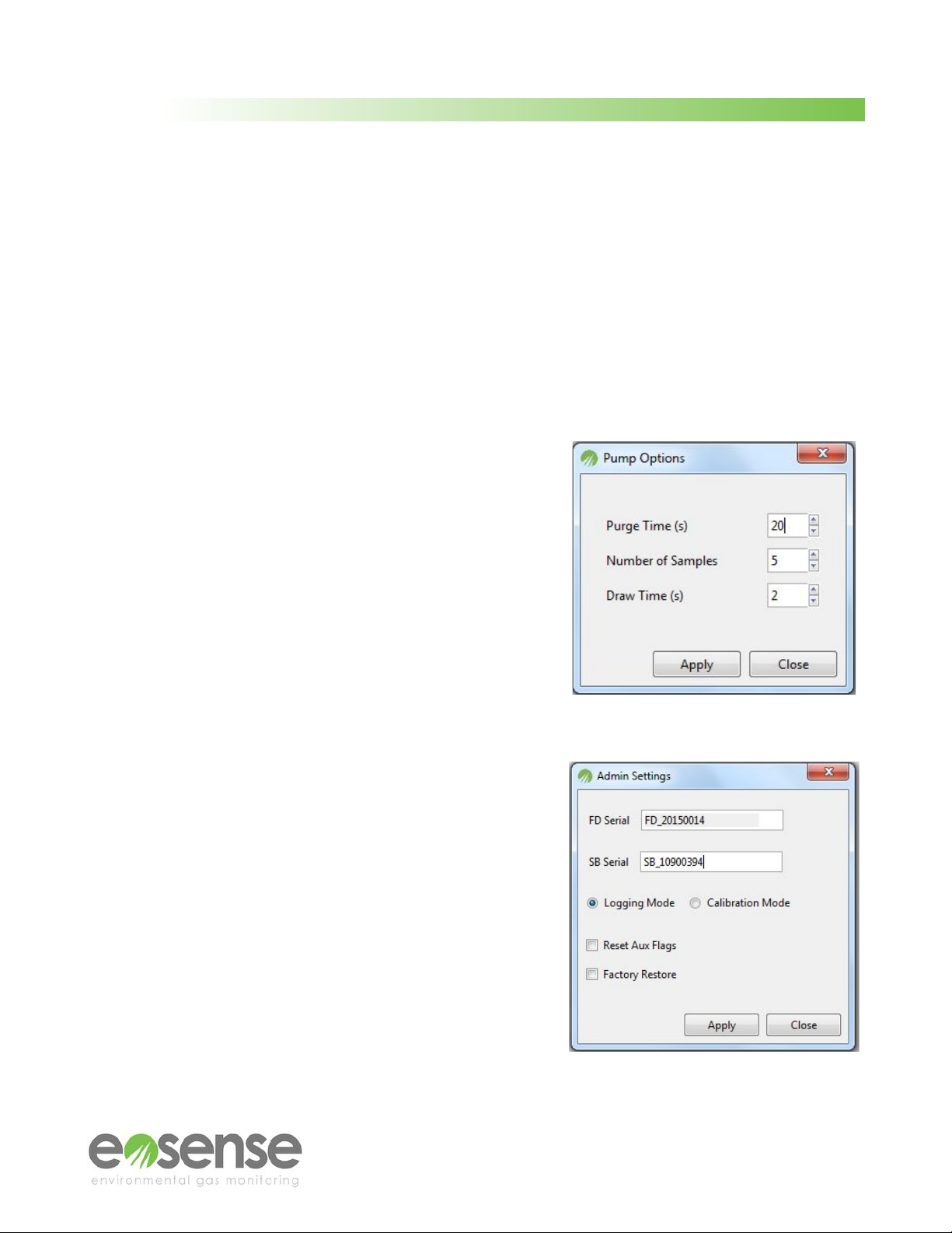
● The Pump Options window allows the user to change
the pump settings used to draw and analyze soil and
atmospheric cavity CO2gas concentrations. Altering
these values may affect the accuracy of measured flux
rates. Purge Time refers to the length of the purge
cycle between atmospheric and cavity samples.
Number of Samples sets the number of concentration
measurements from which the median concentration is
taken. Draw Time controls how long to allow for
pump-transport of gas from a soil or atmospheric cavity
to the sensor for analysis.
Figure 8 The Pump Options window
● The Device Settings window allows the user to
change the eosFD’s operating mode, serial number
and stored calibration. Please contact Eosense for
access to these options if required. Changing these
options may prevent the eosFD from collecting
flux measurements. Logging Mode is the normal
operating mode for the eosFD, while Calibration
Mode allows for recalibration of the internal CO2
sensor. Reset Aux Flags reverts any changes to the
internal diagnostic values, and Factory Restore
reverts any changes made to the eosFD settings,
including calibration parameters and measurement
frequency settings.
Figure 9 The Device Settings window
15 [email protected]m
© Eosense Inc.

User Manual
● The Record Concentrations window has three suboptions; Soil Cavity, Atmospheric Cavity,
and Alternating. These suboptions are convenient for troubleshooting purposes as it allows the
user to directly measure soil, atmosphere or alternating concentrations at a relatively high
frequency. While recording, a pop-up window displays the sampling measurements which
allows the user to monitor the concentrations live. When sampling is complete, the data will
automatically save to the eosLink-FD software folder.
Alternating data will correlate atmosphere and soil concentrations by an identification number
(0 or 1) located in the fourth data column (Figure 10). The Atmospheric Cavity is identified by 0
and Soil Cavity as 1. The four columns of exported data include:
Time Elapsed The time at which the measurement occurred (seconds)
Concentration The soil/atmosphere concentration of CO2 in ppm.
Temperature The approximate internal temperature of the eosFD in °C.
ATM/Soil Identity Atmosphere Identity (0) Soil Identity (1)
Figure 10 Example of eosFD Alternating Cavity Data, viewed as a spreadsheet
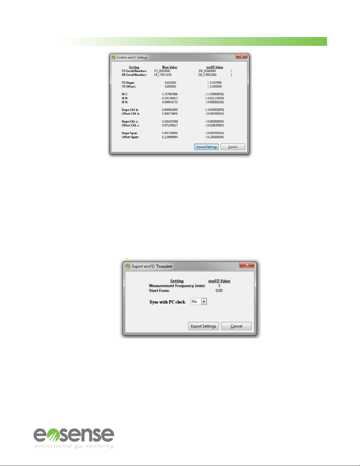
● The eosFD Settings File menu allows a calibration batch file (concentration and flux) to be
uploaded to the eosFD, or exported to a local file. This functionality allows for easy restoration
to factory calibration settings. To export a settings file, choose Export Settings. The eosFD
serial numbers and calibration parameters will be requested from the instrument, and then
displayed in a new window. Clicking the Export Settings will then allow you to choose a location
to save these values for future use.
To upload a settings file, choose Upload File from the menu, and then navigate to a compatible
file (.cal extension). The contained calibration settings will be read in and displayed beside the
current instrument parameters. Click the Upload Settings button to transfer the new coefficients
to the connected eosFD (see Figure 11).
16 [email protected]m
© Eosense Inc.

User Manual
Figure 11 Uploading an eosFD Settings File
●The eosFD Template Files menu allows the user to export eosFD measurement settings as a
local file, which can be used to quickly customize the instrument for different deployment
conditions (e.g. less frequent measurements for off-grid sites) or to standardize settings
amongst multiple eosFDs.
To create a template, choose Export Template from the eosFD Template Files menu, then
choose a save location and filename. The current measurement frequency and start time will be
shown, along with the option to embed a command to synchronize the clock of the eosFD with
the local PC when the template is applied.
Figure 12 Exporting an eosFD Template File
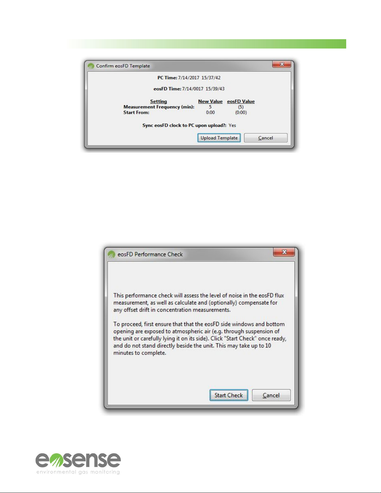
To apply a template file to an eosFD, choose Upload Template from the eosFD Template
Files menu, then navigate to a compatible file (.efd extension). Once the file has been read, the
applicable eosFD measurement settings will be displayed for confirmation. Clicking Upload
Template will apply the frequency and start time settings, and sync the instrument clock with the
local PC (if applicable). See Figure 13 below.
17 [email protected]m
© Eosense Inc.

User Manual
Figure 13 Uploading an eosFD Template File
●The Performance Check option allows the user to assess the atmospheric concentration and
zero flux stability of the eosFD. Choosing this option displays a short explanation of the required
procedure, with the Start Check button used to launch the data collection.
Before proceeding, ensure that the eosFD side windows and bottom opening are exposed to
atmospheric air. For best results, avoid standing directly beside the unit during the Performance
Check.
Figure 14 Starting an eosFD Performance Check test
18 [email protected]m
© Eosense Inc.

User Manual
Once the Performance Check has begun, the eosFD will run through several accelerated
measurement cycles. During this time, the internal pump will operate frequently, as will the
valves. Two progress bars will show the test’s progression.
Figure 15 An eosFD Performance Check in progress
Once the data collection is complete, the results will be presented in two tabs.
Figure 16 Performance Check results for the zero flux
measurements (left) and the atmospheric comparison (right).
The results should show an average flux within 0.2 umol/m2/s of zero under normal conditions,
while the Concentration Results will show an average CO2concentration near 400 ppm.
Differences between the concentration observed by the eosFD (e.g. concentration drift) can be
resolved through the Upload Offset button, though this is not necessary for accurate flux
measurements due to the Forced Diffusion method.
● Admin Mode allows the user to enter a password to enable additional eosFD modifications.
These are not required for normal eosFD operation. Pump Options, Device Settings and
Upload Settings File are restricted to administrator access only. These settings should not
require alteration, however, in special cases where this is necessary please contact
[email protected] for access.
19 [email protected]m
© Eosense Inc.