IMKO SONO-VARIO Xtreme User manual

I:\publik\TECH_MAN\TRIME-SONO\ENGLISH\SONO-VARIO\SONO-VARIO-Xtrem-LD-MAN-Vers2_1-english.doc
SONO-VARIOStandard for general fine Bulk Goods like Sand
SONO-VARIOXtreme for very high abrasive Goods like Gravel and Grit
SONO-VARIOLD for low Density Materials like Grain and Woodchips
IMKO Micromodultechnik GmbH Telefon: +49 - (0)7243 - 5921 - 0
Im Stöck 2 Fax: +49 - (0)7243 - 90856
D - 76275 Ettlingen e-mail: [email protected]
http: //www.imko.de
User Manual
SONO-VARIO

2/44
User Manual for SONO-VARIO
As of 26. June 2013
Thank you for buying an IMKO moisture probe.
Please carefully read these instructions in order to achieve best possible results with your
SONO-VARIO probe for the in-line moisture measurement. Should you have any questions
or suggestions regarding your new probe after reading, please do not hesitate to contact our
authorised dealers or IMKO directly. We will gladly help you.
List of Content:
1. Instrument Description SONO-VARIO...................................................................................... 4
1.1.1. The patented TRIME®TDR-Measuring Method............................................................. 4
1.1.2. TRIME®compared to other Measuring Methods ........................................................... 4
1.1.3. Areas of Application with SONO-VARIOStandard, SONO-VARIOXtrem and SONO-
VARIOLD4
1.2. Mode of Operation................................................................................................................. 5
1.2.1. Measurement value collection with pre-check, average value and filtering................... 5
1.2.2. Determination of the mineral Concentration................................................................... 5
1.2.3. Temperature Measurement............................................................................................ 5
1.2.4. Temperature compensation when working at high temperatures.................................. 5
1.2.5. Analogue Outputs........................................................................................................... 6
1.2.6. The serial RS485 interface............................................................................................. 7
1.2.7. Error Reports and Error Messages ................................................................................ 7
1.3. Configuration of the Measure Mode...................................................................................... 8
1.4. Operation Mode CA and CF at non-continuous Material Flow.............................................. 8
1.4.1. Average Time in the measurement mode CA and CF................................................. 10
1.4.2. Filtering at material gaps in mode CA and CF............................................................. 10
1.4.3. Mode CC –automatic summation of a moisture quantity during one batch process. 11
1.4.4. Mode CH –Automatic Moisture Measurement in one Batch..................................... 13
1.5. Calibration Curves............................................................................................................... 13
1.5.1. SONO-VARIO for measuring Moisture of Sand and Aggregates ................................ 16
1.5.2. SONO-VARIO for measuring Moisture of Expanded Clay and Lightly Sand............... 17
1.6. Creating a linear Calibration Curve for a specific Material.................................................. 18
1.6.1. Nonlinear calibration curves......................................................................................... 19
1.7. Connectivity to SONO Probes............................................................................................. 20
1.7.1. Connection Plug and Plug Pinning............................................................................... 21
1.7.2. Analogue Output 0..10V with a Shunt-Resistor............................................................ 22
1.8. Connection of the RS485 to the SM-USB Module from IMKO............................................ 23

3/44
2. Quick Guide for the Software SONO-CONFIG........................................................................25
2.1.1. Scan of connected SONO probes on the RS485 interface...........................................25
2.1.2. Configuration of Measure Mode....................................................................................26
2.1.3. Analogue outputs of the SONO probe..........................................................................26
2.1.4. Selection of the individual Calibration Curves ..............................................................27
2.1.5. Test run in the respective Measurement Mode ............................................................29
2.1.6. Basic Balancing in Air and Water..................................................................................30
3. Installation of the Probe............................................................................................................31
3.1. Further Assembly Instructions..............................................................................................32
3.2. Assembly Dimensions..........................................................................................................33
3.3. Mounting in curved Surfaces................................................................................................35
3.4. Funnel shape for higher material depth ...............................................................................35
3.5. Gas- and waterproofed Installation ......................................................................................36
3.6. Installation in a conveyor pipeline ........................................................................................37
3.7. Exchange of the Probe Head of the VARIOXtrem/LD .........................................................38
3.7.1. Basic Balancing of a new Probe Head..........................................................................39
4. Technical Data SONO-VARIO...................................................................................................40

4/44
1. Instrument Description SONO-VARIO
1.1.1. The patented TRIME®TDR-Measuring Method
The TDR technology (Time-Domain-Reflectometry) is a radar-based dielectric measuring procedure
at which the transit times of electromagnetic pulses for the measurement of dielectric constants,
respectively the moisture content are determined.
SONO-VARIO consists of a high grade steel casing with a wear-resistant sensor head with ceramic
window. An integrated TRIME TDR measuring transducer is installed into the casing. A high
frequency TDR pulse (1GHz), passes along wave guides and generates an electro-magnetic field
around these guides and herewith also in the material surrounding the probe. Using a new patented
measuring method, IMKO has achieved to measure the transit time of this pulse with a resolution of
1 picosecond (1x10-12), consequently determine the moisture and the conductivity of the measured
material.
The established moisture content, as well as the conductivity, respectively the temperature, can
either be uploaded directly into a SPC via two analogue outputs 0(4) ...20 mA or recalled via a
serial RS485 interface.
1.1.2. TRIME®compared to other Measuring Methods
In contrary to conventional capacitive or microwave measuring methods, the TRIME®technology
(Time-Domain-Reflectometry with Intelligent Micromodule Elements) does not only enable the
measuring of the moisture but also to verify if the mineral concentration specified in a recipe has
been complied with. This means more reliability at the production.
TRIME-TDR technology operates in the ideal frequency range between 600MHz and 1,2 GHz.
Capacitive measuring methods (also referred to as Frequency-Domain-Technology) , depending on
the device, operate within a frequency range between 5MHz and 40MHz and are therefore prone to
interference due to disturbance such as the temperature and the mineral contents of the measured
material. Microwave measuring systems operate with high frequencies >2GHz. At these frequencies,
nonlinearities are generated which require very complex compensation. For this reason, microwave
measuring methods are more sensitive in regard to temperature variation.
SONO probes calibrate themselves in the event of abrasion due to a novel and innovative probe
design. This consequently means longer maintenance intervals and, at the same time, more precise
measurement values.
The modular TRIME technology enables a manifold of special applications without much effort due
to the fact that it can be variably adjusted to many applications.
1.1.3. Areas of Application with SONO-VARIOStandard, SONO-VARIOXtrem and SONO-VARIOLD
SONO-VARIO is suited for moisture measurement of different materials. An installation is possible
into containers, hoppers, above conveyor belts, or in silos.
The SONO-VARIOStandard is suited for measuring of normal abrasive materials like sand and
gravel up to 4mm. The probe head consists of stainless steel with a rectangular ceramic window.
The SONO-VARIOXtrem is suited for measuring of very high abrasive materials like gravel 4/32 and
grit. The probe head consists of hardened steel with a rectangular special ceramic window.
The SONO-VARIOLD (Low Density) is suited for moisture measurement of materials with low
density like corn, wood chips and other materials. For wood chips and other very loose materials
which show a bad flowability, an installation inside a screw conveyor is recommended due to
homogenuous densities inside a screw conveyor.

5/44
1.2. Mode of Operation
1.2.1. Measurement value collection with pre-check, average value and filtering
SONO probes measure internally at very high cycle rates of 10 kHz and update the measurement
value at a cycle time of 250 milliseconds at the analogue output. In these 250 milliseconds a probe-
internal pre-check of the moisture values is already carried out, i.e. only plausible and physically
checked and pre-averaged single measurement values are be used for the further data processing.
This increases the reliability for the recording of the measured values to a downstream control system
significantly.
In the Measurement Mode CS (Cyclic-Successive), an average value is not accumulated and the
cycle time here is 200 milliseconds. In the Measurement Mode CA, CF, CC and CK, not the
momentarily measured individual values are directly issued, but an average value is accumulated via a
variable number of measurements in order to filter out temporary variations. These variations can be
caused by inhomogeneous moisture distribution in the material surrounding the sensor head. The
delivery scope of SONO-VARIO includes suited parameters for the averaging period and a universally
applicable filter function deployable for currently usual applications. The time for the average value
accumulation, as well as various filter functions, can be adjusted for special applications.
1.2.2. Determination of the mineral Concentration
With the radar-based TRIME measurement method, it is now possible for the first time, not only to
measure the moisture, but also to provide information regarding the conductivity, respectively the
mineral concentration or the composition of a special material. Hereby, the attenuation of the radar
pulse in the measured volume fraction of the material is determined. This novel and innovative
measurement delivers a radar-based conductance value (RbC –Radar-based-Conductivity) in dS/m
as characteristic value which is determined in dependency of the mineral concentration and is issued
as an unscaled value. The RbC-measurement range of the SONO-VARIO is 0..12dS/m
1.2.3. Temperature Measurement
A temperature sensor is installed into the SONO-VARIO which establishes the casing temperature
3mm beneath the sensor surface. The temperature can optionally be issued at the analogue output 2.
As the TRIME electronics operates with a power of approximately 1.5 W, the probe casing does
slightly heat up. A measurement of the material temperature is therefore only possible to a certain
degree. The material temperature can be determined after an external calibration and compensation of
the sensor self-heating.
1.2.4. Temperature compensation when working at high temperatures
Despite SONO probes show a generally low temperature drift, it could be necessary to compensate a
temperature drift in special applications. SONO probes offer two possibilities for temperature
compensation.
A) Temperature compensation of the internal SONO-electronic
With this method of temperature compensation, a possible temperature drift of the SONO-electronic
can be compensated. Because the SONO-electronic shows a generally low temperature drift, SONO
probes are presetted at delivery for standard ambient conditions with the parameter TempComp=0.2.
Dependent on SONO probe type, this parameter TempComp can be adjusted for higher temperature
ranges (up to 100°C) to values up to TempComp=0.75. But it is to consider that it is necessary to
make a Basic-Balancing of the SONO probe in air and water, if the parameter TempComp is changed
to another value as TempComp=0.2. The parameter TempComp can be changed with the software
tool SONO-CONFIG, in the menu "Calibration" and the window "TemperatureCompensation".

6/44
B) Temperature compensation for the measured material
Water and special materials like oil fruits and others, can show a dependency of the dielectric
permittivity when using SONO probes at high temperature ranges. The dielectric permittivity is the raw
parameter for measuring water content with SONO probes. If special materials show a very special
temperature drift, e.g. in lower temperatures a higher drift than in higher temperatures, than it could be
necessary to make a more elaborate temperature compensation. Therefore it is necessary to measure
in parallel the material temperature with the temperature sensor which is placed inside the SONO
probe. Normally this is related with high efforts in laboratory works. SONO probes offer the possibility
to set special temperature compensation parameters t0 to t5 for every calibration curve Cal1 of Cal15
(see chapter “Selection of the individual calibration curve”). Please contact IMKO should you need any
assistance in this area.
1.2.5. Analogue Outputs
The measurement values are issued as a current signal via the analogue output. With the help of the
service program SONO-CONFIG, the SONO-VARIO can be set to the two versions for 0..20mA or
4..20mA. Furthermore, it is also possible to variably adjust the moisture dynamic range e.g. to 0-10%,
0-20% or 0-30%. For a 0-10V DC voltage output, a 500R resistor can be installed in order to reach a
0..10V output.
Analogue Output 1: Moisture in % (0…20%, variable adjustable)
Analogue Output 2: Conductivity (RbC) or optionally the temperature.
In addition, there is also the option to split the analogue output 2 into two ranges: into
4..11mA for the temperature and 12..20mA for the conductivity. The analogue output
2 hereby changes over into an adjustable one-second cycle between these two
(current) measurement windows.
For the analogue outputs 1 and 2 there are thus two adjustable options:
Analog Output: (two possible selections)
0..20mA 4..20mA
Output Channel 1 and 2: (three possible selections)
1. Moist, Temp. Analogue output 1 for moisture, output 2 for temperature.
or
2. Moist, Conductivity Analogue output 1 for moisture, output 2 for conductivity in
a range of 0..20dS/m.
or
3. Moist, Temp/Conductivity Analogue output 1 for moisture, output 2 for
both, temperature and conductivity with an automatic current-window change.
For analogue output 1 and 2 the moisture dynamic range and temperature dynamic
range can be variably adjusted. The moisture dynamic range should not exceed
100%
Moisture Range: Temp. Range:
Maximum: e.g. 20 for sand (Set in %) Maximum: 100 °C
Minimum: 0 Minimum: 0 °C

7/44
1.2.6. The serial RS485 interface
SONO-VARIO is equipped with a standard RS485 interface to serially readout individual parameters
or measurement values. An easy to implement data transfer protocol enables the connection of
several sensors/probes at the RS485-Interface. In addition, the SONO-VARIO can be directly
connected to the USB port of a PC, in order to adjust individual measuring parameters or conduct
calibrations, via the RS485 USB Module which can be provided by IMKO.
1.2.7. Error Reports and Error Messages
SONO-VARIO is very fault-tolerant. This enables failure-free operation. Error messages can be
recalled via the serial RS485 interface.

8/44
1.3. Configuration of the Measure Mode
The configuration of SONO-VARIO is preset in the factory before delivery. A process-related later
optimisation of this device-internal setting is possible with the help of the service program SONO-
CONFIG. For all activities regarding parameter setting and calibration the probe can be directly
connected via the RS485 interface to the PC via a RS485 USB-Module which is available from IMKO.
The following settings of SONO-VARIO can be amended with the service program SONO-CONFIG:
Measurement-Mode and Parameters:
Measurement Mode A-On-Request (only in network operation for the retrieval of measurement
values via the RS485 interface).
Measurement Mode C Cyclic:
SONO-VARIO is supplied ex factory with suited parameters in Mode CA with 1 second
average time for bulk goods.
Mode CS: (Cyclic-Successive) For very short measuring processes (e.g. 5…20 seconds)
without floating average, with internal up to 100 measurements per second and a cycle time of
250 milliseconds at the analogue output. Measurement mode CS can also be used for getting
raw data from the SONO-probe without averaging and filtering.
Mode CA: (Cyclic-Average-Filter) For relative short measuring processes with continual
average value, filtering and an accuracy of up to 0.1%
Mode CF: (Cyclic-Float-Average) for continual average value with filtering and an accuracy of
up to 0.1% for very slowly measuring processes, e.g. in fluidized bed dryers, conveyor belts,
etc.
Mode CK: (Cyclic-Kalman-Filter) Standard setting for SONO-MIX for use in fresh concrete
mixer with continual average value with special dynamic Kalman filtering and an accuracy of
up to 0.1%.
Mode CC: (Cyclic Cumulated) with automatic summation of a moisture quantity during one
batch process.
Mode CH: (Cyclic Hold) similar to mode CC but without summation.
Calibration (if completely different materials are deployed)
Each of these settings will be preserved after shut down of the probe and is therefore stored on a
permanent basis.
1.4. Operation Mode CA and CF at non-continuous Material Flow
For mode CA and CF the SONO probes are supplied ex factory with suited parameters for the
averaging time and with a universally deployable filter function suited for most currently applications.
The setting options and special functions of SONO probes depicted in this chapter are only rarely
required. It is necessary to take into consideration that the modification of the settings or the
realisation of these special functions may lead to faulty operation of the probe!
For applications with non-continuous material flow, there is the option to optimise the control of the
measurement process via the adjustable filter values Filter-Lower-Limit, Filter-Upper-Limit and the time
constant No-Material-Keep-Time. The continual/floating averaging can be set with the parameter
Average-Time.

9/44
Parameters in the Measurement
Mode CA, CF and CK
Function
Average-Time
Standard Setting: 10
Setting Range: 1…20
The time (in seconds) for the generation of the
average value can be set with this parameter.
Filter-Upper-Limit-Offset
Standard Setting: 5
Setting Range: 1….20
With the setting of 20, this parameter
must be disabled for Mode CK !
Too high measurement values generated due to
metal wipers or blades are filtered out. The
offset value in % is added to the dynamically
calculated upper limit.
Filter-Lower-Limit
Standard Setting: 2
Setting Range: 1.….20
With the setting of 20, this parameter
must be disabled for Mode CK !
Too low measurement values generated due to
insufficient material at the probe head are
filtered out. The offset value in % is subtracted
from the dynamically calculated lower limit with
the negative sign.
Upper-Limit-Keep-Time
Standard Setting: 5
Setting Range: 1...100
With the setting of 100, this parameter
must be disabled for Mode CK !
The maximum duration (in seconds) of the filter
function for Upper-Limit-failures (too high
measurement values) can be set with this
parameter.
Lower-Limit-Keep-Time
Standard Setting: 30
Setting Range: 1...100
With the setting of 100, this parameter
must be disabled for Mode CK !
The maximum duration (in seconds) of the filter
function for Lower-Limit-failures (too low
measurement values) for longer-lasting
"material gaps", ie the time in which no material
is located on the probe, can be bridged.
Kalman Filter-Parameter in
Measurement Mode CK:
Q-Parameter
Standard Setting: 1x10-5
Setting Range: 0.01…1x10-7
This Kalman filter parameter Qis used to
characterize the systemic measurement error. It
is recommended to leave this parameter to the
default setting!
R-Parameter
Standard Setting: 0.033
Setting Range: 0.01 ….. 0.1
This Kalman filter parameter Ris used for
smoothing the measurement error. The lower
this parameter, the faster is the response to
smaller changes in the moisture readings. The
higher this parameter is the more smoothed the
measured value, but with a delayed reaction
time. It is recommended to leave this parameter
to the default setting!
K-Parameter
Standard Setting: 0.01
Setting Range: 0.01 ….. 0.2
This Kalman filter parameter Kis used for a pre-
dynamic behaviour of the Kalman Filter for
higher changes in the moisture reading, i.e. the
reaction rate of the measurement signal can be
affected hereby. The K-parameter is related to
the Average-Time. It is recommended to leave
this parameter to the default setting!

10/44
1.4.1. Average Time in the measurement mode CA and CF
SONO-VARIO establishes every 200 milliseconds a new single measurement value which is
incorporated into the continual averaging and issues the respective average value in this timing cycle
at the analogue output. The averaging time therefore accords to the “memory” of the SONO-VARIO.
The longer this time is selected, the more inert is the reaction rate, if differently moist material passes
the probe. A longer averaging time results in a more stable measurement value. This should in
particular be taken into consideration, if the SONO probe is deployed in different applications in order
to compensate measurement value variations due to differently moist materials.
At the point of time of delivery, the Average Time is set to 4 seconds. This value has proven itself to be
useful for many types of applications. At applications which require a faster reaction rate, a smaller
value can be set. Should the display be too “unstable”, it is recommended to select a higher value.
1.4.2. Filtering at material gaps in mode CA and CF
A SONO probe is able to identify, if temporarily no or less material is at the probe head and can filter
out such inaccurate measurement values (Filter-Lower-Limit). Particular attention should be directed
at those time periods in which the measurement area of the probe is only partially filled with material
for a longer time, i.e. the material (sand) temporarily no longer completely covers the probe head.
During these periods (Lower-Limit-Keep-Time), the probe would establish a value that is too low. The
Lower-Limit-Keep-Time sets the maximum possible time where the probe could determine
inaccurate (too low) measurement values.
Furthermore, the passing or wiping of the probe head with metal blades or wipers can lead to the
establishment of too high measurement values (Filter-Upper-Limit). The Upper-Limit-Keep-Time
sets the maximum possible time where the probe would determine inaccurate (too high) measurement
values.
Using a complex algorithm, SONO probes are able to filter out such faulty individual measurement
values. The standard settings in the Measurement Mode CA and CF for the filter functions depicted
in the following have proven themselves to be useful for many applications and should only be altered
for special applications.
It is appropriate to bridge material gaps in mode CA with Upper- and Lower-Limit Offsets and Keep-
Time. For example the Lower-Limit Offset could be adjusted with 2% with a Lower-Limit Keep-Time of
5 seconds. If the SONO probe determines a moisture value which is 2% below the average moisture
value with e.g. 8%, than the average moisture value will be frozen at this value during the Lower-Limit
Keep-Time of 5 seconds. In this way the material gap can be bridged. This powerful function inside the
SONO probe works here as a highpass filter where the higher moisture values are used for building an
average value, and the lower or zero values are filtered out. In the following this function is described
with SONO parameters.
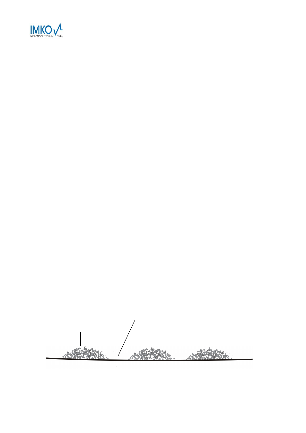
The following parameter setting in mode CA fits a high pass filtering for bridging material gaps.
Sufficient material for an
accurately moisture
measurement value of e.g.8%
Material gaps over e.g. 3 seconds which must
be bridged for an accurately measurement with
a Lower-Limit Keep-Time of 5 seconds.

11/44
The Filter Upper-Limit is here deactivated with a value of 20, the Filter Lower-Limit is set to 2%.
With a Lower-Limit Keep-Time of 5 seconds the average value will be frozen for 5 seconds if a
single measurement value is below the limit of 2% of the average value. After 5 seconds the
average value is deleted and a new average value building starts. The Keep-Time function stops if
a single measurement value lies within the Limit values.
1.4.3. Mode CC –automatic summation of a moisture quantity during one batch process
Simple PLCs are often unable to record moisture measurement values during one batch process with
averaging and data storage. Furthermore there are applications without a PLC, where accumulated
moisture values of one batch process should be displayed to the operating staff for a longer time.
Previously available microwave moisture probes on the market show three disadvantages:
1. Such microwave probes need a switching signal from a PLC for starting the averaging of the
probe. This increases the cabling effort.
2. Time delays can occur during the summation time with a trigger signal which leads to
measurement errors. This is particularly disadvantageous for small batches, recipe errors can
occur.
3. Material gaps during one batch process will lead to zero measurement values which falsify the
accumulated measurement value considerably, recipe errors can occur.
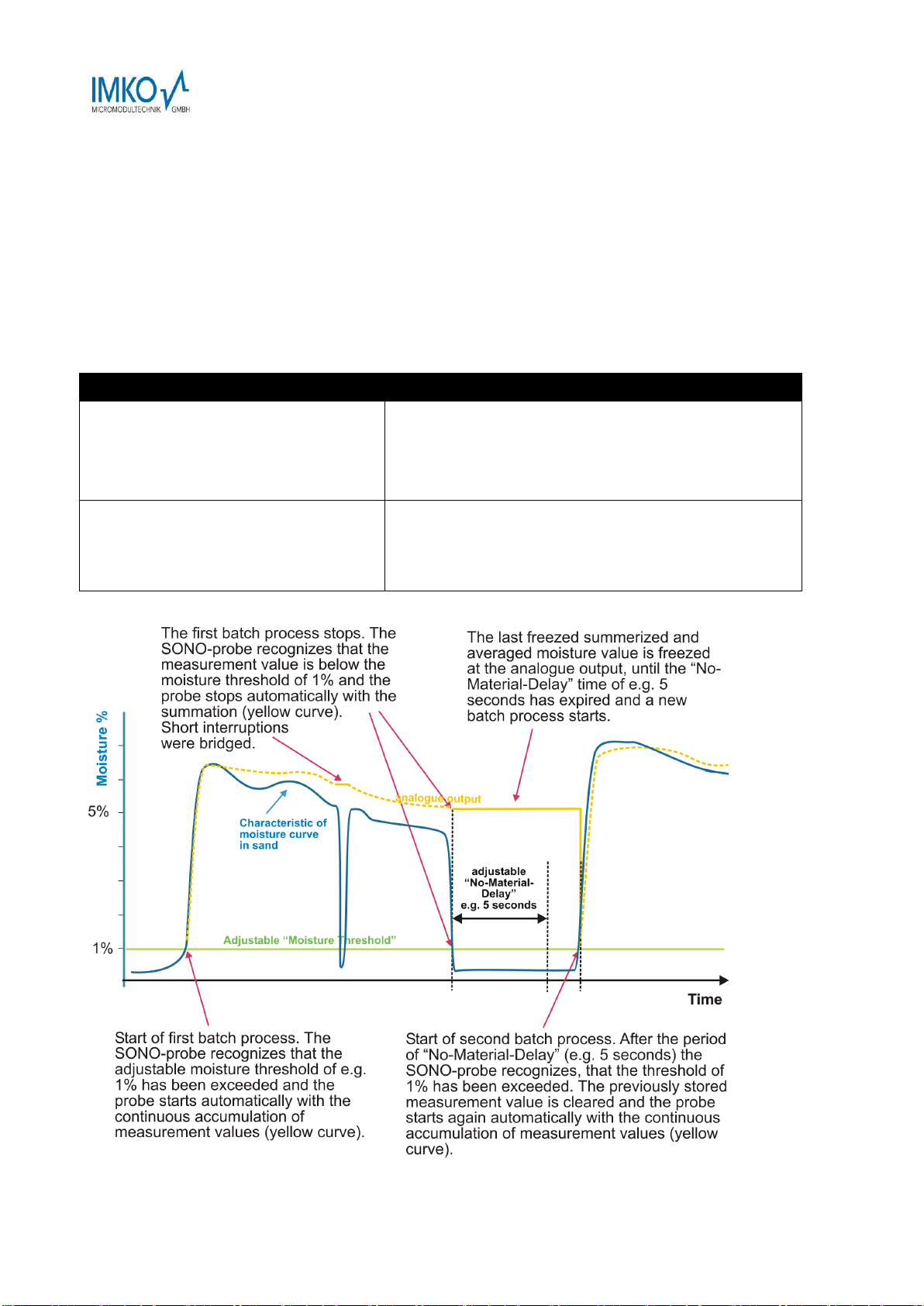
Unlike current microwave probes, SONO probes work in mode CC with automatic summation, where it
is really ensured that material has contact with the probe. This increases the reliability for the moisture
measurement during one complete batch process. The summation is only working if material fits at the
probe. Due to precise moisture measurement also in the lower moisture range, SONO probes can
record, accumulate and store moisture values during a complete batch process without an external
switching or trigger signal. The SONO probe “freezes” the analogue signal as long as a new batch
process starts. So the PLC has time enough to read in the “freezed” moisture value of the batch. For
applications without a PLC the “freezed” signal of the SONO probe can be used for displaying the
moisture value to a simple 7-segment unit as long as a new batch process starts.
With the parameter Moisture Threshold the SONO probe can be configured to the start moisture
level where the summation starts automatically. Due to an automatic recalibration of SONO probes, it
is ensured that the zero point will be precisely controlled. The start level could be variably set
dependent to the plant. Recommended is a level with e.g. 0.5% to 1%.
With the parameter No-Material-Delay a time range can be set, where the SONO probe is again
ready to start a new batch process. Are there short material gaps during a batch process which are
shorter than the “No-Material-Delay”, with no material at the probes surface, then the SONO probe
pauses shortly with the summation. Is the pause greater as the “No-Material-Delay” then the probe is
ready to start a new batch process.

12/44
How can the mode CC be used, if the SONO probe cannot detect the „moisture threshold“ by
itself, e.g. if there is constantly material above the probe over a longer time: In this case, a short
interrupt of the probe´s power supply, e.g for about 0.5 seconds with the help of a relay contact of the
PLC, can restart the SONO probe at the beginning of the material transport. After this short interrupt
the SONO probe starts immediately with the summarizing and averaging.
Please note: It should be noted that no material sticks on the probes surface. Otherwise the moisture
zero point of the probe will be shifted up and the probe would not be detect a moisture low value
below the “Moisture-Threshold”.
Following possible parameter settings in mode CC inside the SONO probe can be set:
Parameter in mode CC
Function
Moisture Threshold
(in %-moisture)
Standard Setting: 1
Setting Range: 1….20
The accumulation of moisture values starts above the
„Moisture Threshold“ and the analogue signal is
output. The accumulation pauses if the moisture level
is below the threshold value.
No-Material-Delay
(in seconds)
Standard Setting: 5
Setting Range: 1….20
The accumulation stopps if the moisture value is below
the moisture threshold. The SONO probes starts
again in a new batch with a new accumulation after the
time span of the “No-Material-Delay” is exceeded.

13/44
1.4.4. Mode CH –Automatic Moisture Measurement in one Batch
If the PLC already accumulates moisture values, than an additional automatic summation of a
moisture quantity inside the SONO-VARIO during one batch process will produce errors.
From the procedure the mode CH is identically with the mode CC, but without automatic summation.
1.5. Calibration Curves
SONO-VARIO is supplied with a universal calibration curve for sand (Cal1: Universal Sand Mix). A
maximum of 15 different calibration curves (CAL1 ... Cal15) are stored inside the SONO probe and
can optionally be activated via the program SONO-CONFIG.
A preliminary test of an appropriate calibration curve (Cal1. .15) can be activated in the menu
"Calibration" and in the window “Material Property Calibration" by selecting the desired calibration
curve (Cal1...Cal15) and with using the button “Set Active Calib”. The finally desired and possibly
altered calibration curve (Cal1. .15) which is activated after switching on the probes power supply will
be adjusted with the button "Set Default Calib”.
Nonlinear calibrations are possible with polynomials up to 5th grade (coefficients m0...m5).
IMKO publish on its website more suitable calibration coefficients for different materials. These
calibration coefficients can be entered and stored in the SONO probe by hand (Cal14 and Cal15) with
the help of SONO-CONFIG.
The charts (Cal.1 .. 15) in the next two pages show different selectable calibration curves which are
stored inside the SONO probe.
Plotted is on the y-axis the gravimetric moisture (MoistAve) and on the x-axis depending on the
calibration curve the associated radar time tpAve in picoseconds. With the software SONO-CONFIG
the radar time tpAve is shown on the screen parallel to the moisture value MoistAve (see "Quick
Guide for the Software SONO-CONFIG). In air, SONO-probes measure typically 60 picoseconds
radar time.

14/44

15/44

16/44
1.5.1. SONO-VARIO for measuring Moisture of Sand and Aggregates
The TRIME-TDR technology with the radar method offers high reliability for measuring moisture of
sand and aggregates, as different grain sizes, unlike other measurement techniques such as
microwave technology, do not cause any distortion of the measurement result.
The calibration curve Cal1 "Universal Sand Mix" is suitable for measuring the moisture in bulk sand,
gravel and gravel/sand granulates. The deviations to the universal calibration curve Cal1 are
approximately +-0.5%, depending on the moisture range, for the below listed gravel/sand types.

17/44
1.5.2. SONO-VARIO for measuring Moisture of Expanded Clay and Lightly Sand
Concerning the material density, expanded clay and lightly sand differ significantly in comparison to
sand and gravel. Therefore a separate calibration for each material is necessary. It is to consider that
expanded clay below a moisture level of 12% still can absorb more water, ie here it must be calculated
with more addition of water into a mixture. At moisture levels above 12% (the maximum core moisture
of expanded clay), the surface water of the expanded clay would act as a free addition of water and
the addition of water into a mixture should be reduced.
For measuring these two materials the probe calibration Cal10 or Cal11 can be selected.
If you want to use a single SONO probe with the calibration Cal1 for both normal sand/gravel as well
as these two materials, then there is the possibility with a simple mathematical conversion inside a
PLC. Requirement would be that the PLC knows when and what material is to be measured. You may
convert the following:
MoistureLightlySand = MeasurementValueCal1 * Factor of 4
MoistureExpandedClay = MeasurementValueCal1 * Factor of 4.8 + 3.2 Offset
It is to consider that this correction calculation for expanded clay can only be measured above 3.2%,
which in practice would be acceptable as it is unlikely that in plant operation the moisture in expanded
clay is below 3.2%.

18/44
1.6. Creating a linear Calibration Curve for a specific Material
The calibration curves Cal1 to Cal15 can be easily created or adapted for specific materials with the
help of SONO-CONFIG. Therefore, two measurement points need to be identified with the probe.
Point P1 at dried material and point P2 at moist material where the points P1 and P2 should be far
enough apart to get a best possible calibration curve. The moisture content of the material at point P1
and P2 can be determined with laboratory measurement methods (oven drying). It is to consider that
sufficient material is measured to get a representative value.
Under the menu "Calibration" and the window "Material Property Calibration" the calibration curves
CAL1 to Cal15 which are stored in the SONO probe are loaded and displayed on the screen (takes
max. 1 minute). With the mouse pointer individual calibration curves can be tested with the SONO-
probe by activating the button "Set Active Calib". The measurement of the moisture value
(MoistAve) with the associated radar time tpAve at point P1 and P2 is started using the program
SONO-CONFIG in the sub menu "Test" and "Test in Mode CF" (see "Quick Guide for the Software
SONO- CONFIG").
Step 1: The radar pulse time tpAve of the probe is measured with dried material. Ideally, this takes
place during operation of a mixer/dryer in order to take into account possible density fluctuations of the
material. It is recommended to detect multiple measurement values for finding a best average value
for tpAve. The result is the first calibration point P1 (e.g. 70/0). I.e. 70ps (picoseconds) of the radar
pulse time tpAve corresponds to 0% moisture content of the material. But it would be also possible to
use a higher point P1´ (e.g. 190/7) where a tpAve of 190ps corresponds to a moisture content of 7%.
The gravimetric moisture content of the material, e.g. 7% has to be determined with laboratory
measurement methods (oven drying).
Step 2: The radar pulse time tpAve of the probe is measured with moist material. Ideally, this also
takes place during operation of a mixer/dryer. Again, it is recommended to detect multiple
measurement values of tpAve for finding a best average value. The result is the second calibration
point P2 with X2/Y2 (e.g. 500/25). I.e. tpAve of 500ps corresponds to 25% moisture content. The
gravimetric moisture content of the material, e.g. 25% has to be determined with laboratory
measurement methods (oven drying).
Step 3: With the two calibration points P1 and P2, the calibration coefficients m0 and m1 can be
determined for the specific material (see next page).
Step 4: The coefficients m1 = 0.0581 and m0 = -4.05 (see next page) for the calibration curve Cal14
can be entered directly by hand and are stored in the probe by pressing the button “Set”. The name of
the calibration curve can also be entered by hand. The selected calibration curve (e.g. Cal14) which is
activated after switching on the probes power supply will be adjusted with the button "Set Default
Calib”.
Attention: Use “dot” as separator (0.0581), not comma !

19/44
1.6.1. Nonlinear calibration curves
SONO probes can also work with non-linear calibration curves with polynomials up to 5th grade.
Therefore it is necessary to calibrate with 4…8 different calibration points. To calculate nonlinear
coefficients for polynomials up to 5th grade, an EXCEL software tool from IMKO can be used (on
request). It is also possible to use any mathematical program like MATLAB for finding a best possible
nonlinear calibration curve with suitable coefficient parameters m0 to m5 which can be entered into the
probe with help of SONO-CONFIG.
The following diagram shows a sample calculation for a linear calibration curve with the coefficients
m0 and m1 for a specific material.

20/44
1.7. Connectivity to SONO Probes