Bridgeport MCA-3000 User manual

Bridgeport Instruments, LLC, 11740 Jollyville Rd., Ste 500, Austin, TX 78759,
www.BridgeportInstruments.com
By Michael Momayezi
Phone [phone]
Fax [phone]
email momayezi
@bridgeportinstruments.com
MCA-3000 Users Manual
V 3.2, June 2021
Summary
The MCA-3000 is a family of high-performance multi-channel analyzers (MCA) for measuring
gamma-ray radioactivity with a scintillator.
The PMT-3000 includes a operating voltage supply and plugs directly onto a photomultiplier.
The SiPM-3000 includes the SiPM operating voltage supply and plugs directly onto an SiPM-array.
Using its embedded 32-bit ARM processor, it provides accurate gamma-ray spectroscopy and gain
stabilization together with many advanced features such as automatic background subtraction and
alarm computations.
This document describes how to use the MCA-3000 from the graphical user interface and from
Python scripts. Using the MCA Data Server, developers will find they can program the MCA-3000
in any language they want.
Feature summary – PMT-3000
More than 4Mcps histogramming rate
Suitable for all scintillators via programmable integration time
Positive and negative operating voltage and different PMT pinouts.
Feature summary – SiPM-3000
Suitable for 500kcps on NaI(Tl) or faster scintillators
Suitable for many scintillators via programmable integration time
Very low-noise integrated SiPM voltage supply
Very low trigger threshold: <10keV with 2MeV energy range.
Feature summary – Common characteristics
Histogram: 4K×32; Loss-less two-bank mode with 2× 2K×32;
List mode, pulse shape capture
On the fly pulse shape discrimination
Built-in programmable gain stabilization performed by embedded ARM processor
USB interface; Serial interface on PCB; default 115200 baud
FPGA customization possible for application specific product
ARM C-code customization possible for application specific product
Power consumption is only 300mW (5V@60mA)
Popular FPGA firmware options
Loss-less dual bank list mode buffer with 2047 events per buffer.
100ms time slice operation with 20-deep buffer, events and 1k histogram per slice.
Popular software options

Sample vs background measurements with alarm computation
Radiation Portal mode with automatic background tracking and programmable alarm

Table of Contents
1. Supporting Documentation
2. Getting Started
3. Energy Spectrum
4. Calibration
5. Gain Stabilization
6. Summation Weights
7. Pulse Shape Discrimination
8. Analog
9. Mechanical and Pin Outs
10. Ordering
1. Supporting Documentation
Open-source software The software is open
source and mostly written in Python.
Bridgeport Instruments provides a software
installer, which by default will create a
C:\BPISoftV3 directory. That folder includes
Python 3.7 with three added packages: ZMQ
(www.zeromq.net), wxPython and Matplotlib v
3.2. ZMQ is used to implement the client-
server behavior and it is accessible from more
than 40 programming languages. Matplotlib is
used for the graphics interface, and wxPython
is used to create a traditional user interface
with pull down menus.
The wxMCA folder that contains the MCA
software can be placed anywhere on the hard
disk. Inside is a folder called documentation
and the best starting page is
wxMCA/documentation/english/
introduction/introduction.html which you can
open in any web-browser. This set of linked
documents contains a description of every
control variable and every data field used by
the MCA-3000.
2. Getting started
2.1 Using the USB interface
For USB communication the MCA-3000 uses
libusb0.1 (Linux) and libusb_win32 on
Windows 10. The Windows 10 libusb dll is
digitally signed. When the MCA hardware is
present during the installation, the installer will
automatically link the MCA-3000 to
libusb_win32.
However, it is also possible to simply copy the
BPISoftV3 folder onto the C: drive and install
the Windows USB-driver manually. This needs
to be done only once, and Windows will later
recognize any other MCA-3000, by its USB
vendor ID of 0x1FA4 and the USB product ID
of 0x0103 (PMT-3000) or 0x203 (SiPM-3000).
Open the Windows Device Manager and
connect the MCA-3000 to a USB port. Wait
until it appears in the Device Manager as an
unknown device of type armMorpho or
sipmMorpho.
Open the C:\BPISoftV3 folder and launch
zadig-2.4.exe. Use Options/ListAllDevices to
refresh the device list and select the select the
device with the BPI vendor ID of 0x1FA4. To
the right of the green arrow, select libusb-
win32(v1.2.6.0) and click the big
'InstallDriver' button below. Note that it may
take up to 20 seconds for the screen to update -
be patient. Once the 'Driver Installation
Successful' message appears you can close the
window. In the Device Manager you will now
see the MCA-3000 listed under 'libusb-win32
devices'.
2.2 Launching the software
First launch the MCA Data Server. Look
inside the wxMCA folder. Under Windows,
double-click on run_mds.cmd. Under Linux,
launch wxMCA/mds/mds_server.py making
sure you use a python 3.7 or higher installation
that also includes ZMQ, wxPython and
Matplotlib.
If the MDS reports no MCA found, the OS
may have been slow in enumerating the MCA
on the USB bus. Kill the MDS and launch it
again.
Then launch the User Interface. Under
Windows, double-click on run_wxMCA.cmd.
Under Linux, launch
wxMCA/wxGUI/MCA_Main.py
The items in the menu bar are mostly self-
explanatory. You can view results and edit
instrument settings in a spread-sheet
environment. To send the changed values to the
instrument, you need to click on File
→toMCA.
3. Energy Spectrum
The MCA provides fast and accurate
measurements of energy spectrum and count
rates. To acquire an energy histogram, select
Display→Histogram from the menu bar. In
response, a histogram panel will open. On that
panel use "New" to erase the old histogram and

count rate data and begin a new acquisition.
The panel does not automatically refresh, so
click the "Refresh" button to get an updated
energy spectrum.
Use Save to append the energy histogram
and count rate data to a data file.
3.1 Adjusting operating voltage
You need to set the electronic gain and
adjust the operating voltage to set the
maximum measurable energy.
Then adjust the digital gain to achieve the
desired MCA calibration in keV per bin
The maximum measurable energy is
independent of the number of histogram bins
used. Users need to adjust the operating voltage
to change the gain of the SiPM or PMT. In the
table below we recommend maximum
measurable energies for different applications.
Max.
Energy Comment
1.0MeV
High gain for measuring low energies down to
20keV. Good for measuring contamination with
Cs-137 and Cs-140 (fresh fission product), or
Radium isotopes.
2.0MeV Measure NORM up to K-40 at 1460keV
3.0MeV Wide range covers all naturally occurring
gamma-rays, even to Tl-208 at 2615keV
Table 1: Cs-137 calibration for different tasks; NORM:
Naturally occurring radioactive materials
How to determine the maximum measurable
energy. In the fpga_ctrl  display set
ha_mode  to 1 to measure the pulse height.
The maximum measurable pulse height is 900.
Start a new histogram and record the peak
position (P) of a known isotope; eg E=662keV
of Cs-137. The maximum measurable energy is
computed as
Hence, putting the pulse height peak of Cs-137
at 187mV will result in a maximum measurable
enery of 3.18MeV.
There are four discrete electronic gains that can
be applied. In fpga_ctrl , select gain_select
= 1, 2, 4, or 8 for increasingly higher electronic
gains. Note that the highest electronic gain will
slow down the input amplifier response and is
usually only used for slow scintillators, such as
CsI(Na).
For a continuous and smooth gain change,
vary the operating voltage to move the pulse
height peak. Access the operating voltage
control by opening the arm_ctrl  display.
Enter a new operating voltage in the cal_ov
field and hit enter. Use File→ToMCA to write
the voltage to the MCA.
Go back to the Histogram  display and click
New  to start a new acquisition. If you change
the operating voltage by 1%, the PMT gain will
change by about 6%. For the SiPM-3000 the
gain equation is
Once the pulse height peak is in the right
position and therefore the maximum energy has
been set, keep the operating voltage and the
electronic gain constant.
Now adjust the digital gain to achieve the
desired MCA calibration in keV per bin.
Once the operating voltage has been
established, set ha_mode back to 0, and start
a new histogram
Determine the measured peak position (P) and
use the desired peak position (E) to determine
the new digital_gain
With that the detector has been calibrated. See
the calibration section 4 for a much more
detailed description.
3.2 Count rate measurement
Observe how the count rate accuracy
improves with measurement time. The MCA
reports count rates together with their statistical
errors. This gives users a useful tool. Manually,
or programmatically, they can end a
measurement precisely when the desired
accuracy has been reached, which saves time
and money.
The error (in %) is computed from the number
of events as 100×2/sqrt(N), where N is the
number of events. This is called the statistical
2-σ error. The true count rate lies within this
error range with a 95% probability.
Note that the MCA corrects the recognized
count rate using the known dead time per
event. Hence the reported count rate is greater
than the recognized count rate. The reported
count rate is also an accurate estimate of the
true number of counts per second. In fact the
reported count rate should match the true input
count rate with about 1% accuracy (systematic
error) for input count rates up to 100kcps. The
statistical count rate error is computed correctly
using the number of recognized events.
= E ⋅
E
max
900
P
gain = 1.0e6 ⋅ ( V − 28.6V)
= g ⋅
g
new
E
P

3.3 Histogramming speed
The MCA has a non-extendable dead time
equal to the hold_off_time per recognized
event. For NaI(Tl) between 5°C and 65°C the
MCA-3000 recommends a fixed hold off time
for NaI of 1.2µs. The resulting throughput is
shown in the next figure.
Fig. 1: Expected histogramming rate vs input count
rate for a hold_off_time = 1.2µs; (ie typical for NaI(Tl)
at room temperature.
The SiPM-3000 will match the speed of the
PMT-3000 for NaI. For LaBr3 the PMT-3000
can go even faster – at a fixed hold off time of
only 0.3µs. The resulting throughput is shown
in the next figure.
Fig. 2: Expected histogramming rate vs input count
rate for a hold_off_time = 0.3µs; (ie typical for LaBr3.
3.4 High count rates
There may be a small gain shift at high
count rates. Users should be aware that at
input count rates above a few 10kcps there may
occur small gain shifts in the energy spectrum.
Typically, at 50kcps the gain may fall by about
1%, but the exact gain shift will depend on the
PMT that is used on the detector.
4. Calibration
4.1 Theory of operation
The MCA-3000 uses a switched-gain input
amplifier stage followed by an ADC with a 1V
input range. The ADC samples the amplifier
output voltage at a rate of typically 40MSPS.
In the PMT-3000, the sampling rate can reach
120MHz.
For proper operation, the amplifier output
voltage must fall within the 1.0V input range of
the ADC, as shown in the two figures below.
Fig. 3: A regular NaI(Tl) pulse.
Fig. 4: An out of range NaI(Tl) pulse. Note how it
cannot reach beyond 1023mV.
Pulse height is a measure of the difference
between the maximum pulse voltage and the
baseline from which it rises.
There is a built-in DC-offset of around 128mV
and the maximum measurable voltage is shown
as 1.023V. Hence the maximum practical signal
pulse height range is around 900mV.
The first step of calibration at a chosen
electronics gain, is to make sure that the
maximum wanted energy can be measured by
the ADC. At a fixed electronics gain, the
applied operating voltage will determine the
maximum measurable energy.
A very common calibration is to set the
operating voltage such that the full-energy peak
of Cs-137 (661.66keV) corresponds to a pulse
height of 187mV. The maximum measurable
energy is then
900mV/187mV×662keV=3.18MeV.

After adjusting the high voltage to set the
maximum measurable energy, the user can now
vary the digital gain to map the entire energy
spectrum into an energy histogram of the
desired size and calibration.
For example, we assume 40MHz ADC
sampling rate and the recommended integration
time of 1.2µs for NaI(Tl). We also assume that
the Cs-137 662keV peak has an average pule
height of 187mV. In that case, choose a digital
gain of 4700 to place the peak in the energy
histogram at 662keV, ie have an MCA
calibration of 1.0keV per bin.
Below we describe the calibration steps in
detail.
4.2 Calibration file
Calibration controls are in autocal.json. This
file can be found in the
./rad_config/Matplotlib_gui/config/ folder. Its
contents are explained in the table below.
Variable Description
cal_energy The energy, in keV, for the calibration
peak; eg 662 for Cs-137.
cal_pulse_height
The pulse height for the calibration
peak; eg 187 for Cs-137 and 3.2MeV
maximum measurable energy.
auto_update
0→ Off; 1→ Apply the new operating
voltage and restart the mcaafter user
clicks on "Calibrate" button.
keV_bin Desired MCA calibration, as keV per
MCA bin.
gain_exp
PMT's have a power law for their gain
vs voltage function:
Typical values are 5.6 for R6231, 6.0 for
CR105 and 7.5 for many other 10-stage
PMT. For SiPM this parameter is
ignored.
mass
The mass of the NaI crystal, in kg; used
for computing the deposited dose rate
from the count rate and deposited
energy.
Fig. 4: The autocal.json data explained.
For use with Broadcom SiPM we use the
following gain formula:
The 28.6V are the sum of the typical 27V break
through voltage and the 1.6V offset of the
SiPM-3000 input amplifier.
You can manually calibrate the detector, in
which case you have more freedom on how to
do it. If you want to use the Calibrate 
button on the Histogram  panel, then the
software will always pick the tallest peak in the
histogram, beyond 50 MCA bins, to use in the
calibration computations. This works best for
isotopes with a well-separated medium-energy
peak; eg Cs-137 and Na-22. Co-60 is not
recommended for the software-assisted
calibration.
4.3 Step 1 of the calibration
First, adjust the operating voltage to set the
maximum measurable energy. Open the
fpga_ctrl  display and set the ha_mode 
control to 1. Start a new histogram acquisition
on the Histogram  display by clicking on
New . Wait until there are around 1000
counts in the peak maximum. Then click
Calibrate  on the Histogram  display.
After 1 second, you will receive a message
with the suggested new operating voltage. The
software has applied the new operating voltage
already if auto_update is set to 1.
There is some variation between the SiPM or
PMT and you may have to repeat a second time
to achieve the desired accuracy. Note that even
if you do not know the exact gain exponent of
your PMT, the process will still converge. It
may just take another iteration or two.
Here is how to compute the cal_pulse_height
(cph) :
4.4 Step 2 of the calibration
Now change the digital gain to achieve the
desired MCA calibration in keV per MCA
bin.  From here on, the operating voltage and
the electronic gain gain_select should be kept
constant. Instead we use the digital_gain from
the fpga_ctrl  display.
Set the ha_mode  control to 0 to return to
normal energy measurements, and start a new
histogram acquisition. Wait for sufficient
accuracy and click Calibrate .
This time, you will receive a notice of the new
digital_gain .
The new value was computed from a linear
formula
=
gain
gai
n
0
( )
HV
H
V
0
gain_exp
gain = 1.0e6 ⋅ ( V − 28.6V)
cph = 900 ⋅
cal_energy
E
max
= g ⋅
g
new
cal_energy
E
peak

and it will be accurate on the first try.
However, keep in mind that there is a statistical
uncertainty in determining the actual energy of
the histogram peak. You can compute the 1-σ
error from the fwhm (in %) and the number of
net counts (N) above background in the peak as

5. Gain Stabilization
All MCA-3000 offer gain stabilization that
keeps the gain, the trigger threshold and the
maximum measurable energy constant.
NaI(Tl) is the most commonly used scintillator,
and it also one of the most challenging. Its
brightness and pulse shape change with
temperature, while the application engineer
wants to keep constant not only the MCA gain
(keV per bin) but also the trigger threshold and
maximum measurable energy that is
independent of temperature.
All MCA-3000 offer a user-programmable set
of lookup tables to change the operating
voltage and the digital gain to achieve this
goal. In addition, for NaI(Tl) the MCA also
vary the hold-off time with temperature to
avoid retriggering on the tail end of the same
pulse.
Since code and data needed for the gain
stabilization are embedded in the MCA, no
user software is required and the calibration
moves with the detector.
The PMT-3000 also offers LED-based gain
stabilization to counter PMT aging. Vacuum
photomultiplier tubes lose gain over time, even
under light to moderate loads. For example the
popular R6231 PMT loses half its gain after an
accumulated anode charge of about 50C.
Distributed over one year, this equivalent to an
average anode current of just 1.6µA, with a 6%
gain loss per month. With a built-in LED that
injects light into the back of the
photomultiplier, the PMT-3000 can gain-
stabilize on the LED response and counteract
the PMT aging.
5.1 General theory of operation
All types of gain stabilization use lookup
tables, and users can supply their own. The
standard code includes a 64-long float array
with three look up tables (LUT). The MCA
frequently determines the temperature and
adjust the operating parameters according to
the values found in the lookup tables.
The LUT depend on the scintillator and on
one DSP setting, namely the integration
time. For NaI(Tl) the LUT supplied by the
factory use an integration time of 1.2µs. For
the PMT-3000 and NaI(Tl) the LUT supplied
by the factory was derived for an integration
time of 1.2µs. That value remains fixed over
the entire temperature range, as it provides the
best energy resolution for small and large
energies at all temperatures. For the SiPM-
3000 and NaI we suggest a fixed integration
time of 1.5µs.
But the hold-off time has to be varied.
NaI(Tl) pulses become very long when the
crystal temperature falls below 0°C.
Consequently, the hold-off time has to be
increased at low temperatures to avoid
retriggering on the tail end of the same pulse.
Since this phenomenon is determined by the
scintillator physics, it has been implemented as
an immutable function in the MCA, instead of
a lookup table. The function is used if
arm_ctrl["fields"]["cal_scint"]==1.
The implemented hold-off vs time function for
NaI(Tl) is
in µs and with being the temperature in °C.
How the LUT are constructed. Developers
may find that they need to construct the correct
LUT for their detectors, as they may use a
different scintillator or a different PMT. To this
end the detectors needs to be run through a
temperature cycle. The detector is recalibrated
to desired specification at each temperature and
the operating voltage, digital gain and possibly
the LED value are recorded. Using
interpolation one then constructs the LUT at
the fixed temperature steps.
Keep in mind that many crystals don't allow for
rapid temperature changes or they will crack.
10°C per hour is a safe bet for a 50mm NaI.
Secondly, it takes a while for a detector to
attain steady state. The vacuum PMT needs an
hour and the crystal characteristic time depends
on the material and the size. For a 50mm NaI it
takes about half an hour, for a 76mm NaI it
takes 1.5hrs. Hence, it is necessary for a
precise measurement, to maintain the detector
at a fixed temperature for 2 to 4 hours before
moving to the next.
Thermal equilibrium is necessary. Keep in
mind that the PMT and the scintillator both
have different temperature coefficients. If the
two are not in equilibrium, there is no easy way
to provide gain stabilization. Hence an outdoor
ε =
fwhm
2.3655 ⋅
N
−−
√
max(1.25, (0.634 + 1.27 ⋅ exp(− T /32.26)))
T

detector should be packaged with good thermal
insulation to achieve thermal time constants of
2 hours or more – to ensure that all components
are in a steady state situation. However, care
must be taken not to insulate the electronics.
Even if it only dissipates 300mW, that small
amount of power stills needs to drain away to
avoid self heating.
When using SiPM: SiPM-based systems react
more quickly, because the SiPM-array has very
little thermal mass. In uncooled systems its
temperature may be close to the crystal or
halfway between the electronics temperature
and the crystal temperature, depending on the
assembly.
In cooled systems the SiPM-array is well
insulated from the crystal and its temperature
remains constant as long as the Peltier cooling
loop remains in regulation.
As a result, insulation for SiPM-based systems
needs to be, at the minimum, just good enough
to avoid cracking the crystal through
temperature shock.
arm_cal registers and fields
Index:
name Description
0: lut_len Number of entries in the LUT; default is 19,
2..19 are allowed
1:
lut_tmin
Minimum temperature in the lookup table;
Typically -30°C
2: lut_dt Temperature step size in the lookup table;
Typically 5°C
[3:22]:
lut_ov Change of operating voltage vs temperature
[23:42]:
lut_dg Change of digital gain vs temperature
[43:62]:
lut_led Change of LED target vs temperature
63:
lut_mode
int(lut_mode)&0x1 → lock bit, set to 1 to
prevent the user from reading the arm_cal data
from the MCA.
The arm_cal registers and fields.
5.2 Gain stab. summary
Standard software recognizes these gain
stabilization modes (gsm):
0 ⇒ Off; Use when calibrating a detector.
7 ⇒ Suspend; Keep all parameters as they
are.
1 ⇒ Use temperature lookup for change of
operating voltage and digital gain; adjust
hold-off if required.
2 ⇒ Compare measured LED value to
expected value and adjust operating voltage
accordingly. Use LUT for digital gain and
compute hold-off time as needed.
arm_ctrl for detector calibration
Name gsm Description
cal_ov 0,1,2 Operating voltage when the detector
was calibrated
cal_temp 1,2 Temperature (in deg C) at which the
detector was calibrated
cal_dg 1,2 Digital gain when the detector was
calibrated
cal_scint 1,2 Scintillator type; 1⇒ NaI(Tl), adjust
hold-off time vs temperature.
cal_target 2 Target value for response to LED; used
with gain_stab=2
The arm_ctrl registers and fields concerning detector
calibration; The gsm column lists the gain stablization modes
for which this parameter is used.
LUT needed for detector calibration
Name gsm Description
lut_ov 1 Operating voltage
lut_dg 1,2 Digital gain
lut_led 2 LED average
The lookup tables (LUT) needed detector calibration; The
gsm column lists the gain stabilization modes for a given
LUT is used.
5.3 Gain stab. mode: gsm = 0
Off. Gain stabilization is turned off and the
target operating voltage the MCA will set is the
one requested in arm_ctrl["fields"]["cal_ov"].
5.4 Gain stab. mode: gsm = 7
Suspend. This is different from gsm=0. During
the gain stabilization algorithm may
have changed the target operating voltage to a
temperature dependent value that is different
from arm_ctrl["fields"]["cal_ov"]. Setting
gsm=0 would revert to that original value,
while gsm=7 will leave the value unchanged.
The same applies to the digital gain and the
hold-off setting.
5.5 Gain stab. mode: gsm = 1
gsm ≠ 0

This mode relies on just the look up tables
and the measured temperature. It is
implemented for all MCA-3000. The units ship
with LUT determined for NaI(Tl) at an
integration time of 1.25µs
5.6 Gain stab. mode: gsm = 2
This mode adjusts the voltage using an LED
measurement It is only implemented for the
PMT-3000 series. The units ship with LUT
determined for NaI(Tl) at an integration time of
1.25µs
The driving circuit for the LED used in the
gain stabilization is electronically temperature
compensated, but the compensation is not
perfect. Since also the scintillator brightness
changes with temperature, the ratio of the LED
value and the full energy peak from a gamma-
ray will be temperature dependent. Hence,
there needs to be a lookup table to tell by how
much the LED target value needs to be shifted
as the temperature changes, in order to keep a
full-energy gamma-peak constant.
Use an LED when expecting PMT aging. The
purpose of the LED is to counteract PMT
aging. This applies mostly to remotely installed
detectors where a frequent recalibration is not
possible. Whenever a detector can be
recalibrated monthly and only sees light to
moderate loads (anode current < 1µA with
round the clock operation), then an LED
system is not required.
Since aging is not a concern for SiPM, the
SiPM-3000 series does not offer an LED
option.
Adjusting the LED. In the LED panel you will
find the controls shown in the table below
LED controls
Name Description
Period LED frequency =
Width Driver pulse width =
Attenuate Attenuation factor =
On 0→ Off; 1→ On;
Select 0→ LED pulses are hidden; 1→ Only show
LED in histogram and traces
The LED controls.
Manual vs algorithmic operation of the
LED. When gain stabilization is off the user
can set the LED frequency and pulse width.
When the detector has been calibrated, read the
LED value from the RR_10 field on the
fpga_status display and enter it into the
cal_target field on the arm_ctrl display.
Don't run the LED too fast. Keep in mind
that the LED pulses also cause a load on the
PMT which may reduce its gain slightly (1% to
5% worst case). Hence, keep the LED running
at ≤ 100Hz (P>24) during calibration. The
PMT-3000 will update the measured LED
average every 1024 pulses. At a rate of 100Hz,
it will take 10s between updates.
Keep the LED pulses short, especially for
high count rates. When using Select=1 , you
can see the LED values histogrammed. Mostly
they will fall into a narrow peak of with an
"energy resolution" of 1% to 2% fwhm. At
high input count rates from a source (> 20kHz)
you will also see a small fraction of events
classified as LED that are a pile up of an LED
pulse with a gamma-ray. These are rare, but
they do slightly affect the accuracy of the LED
average measurement. Keeping the LED pulses
short helps to suppress these unwanted events.
The LED pulse is shorter than the drive
pulse. Not only is the LED light pulse about
0.9µs shorter than the driver pulse, the FPGA
logic also begins measuring the LED light only
1.5µs after the drive pulse starts. Hence if you
set the LED width W<30 you will see a
measured LED average of zero.
Similarly, the FPGA stops measuring the LED
light about 0.15µs before the pulse actually
ends. These two measure ensure that the LED
light intensity is only measured during the flat
top of the pulse where the behavior is most
predictable.
Usually the pulse height is adjusted at the
factory to about 200mV when the detector is
calibrated to have a maximum energy range of
3.2MeV. This allows operation with a higher
gain and a lower energy range of down to
1MeV max, while keeping the LED pulse
within ADC range.
2441Hz/( P + 1)
W ⋅ 0.050 μ s
1/
2
A

Fig. 5: A wide LED pulse to demonstrate how it is being
measured.
5.7 Dynamical performance for gsm = 2
The gain error falls to < 1% in 10s. If an
instrument that was calibrated at room
temperature is left in a hot vehicle and turned
on at a temperature much different from the
calibration temperature, its initial gain settings
will be all wrong for the new temperature. For
gsm=1 the adjustment will be immediate, as the
instrument only requires one temperature
lookup to adjust to the new situation.
For LED-based gain stabilization (gsm=2)
there is a short time lag. The instrument needs
to measure the new LED value and then step
by step adjust the high voltage to make the
LED value meet the computed LED target. As
shown in the figure below, this process takes
less than 10 seconds. In the beginning the LED
blinks at 1220Hz, and the high voltage is
updated about every 0.8s. Once the LED value
is close to the LED target (within 1%) The
instrument gradually reduces the LED blinking
frequency to 19Hz to reduce the load on the
PMT and avoid accelerated PMT-aging.
This is the response of the gain stabilization algorithm to
turning on the detector at a temperature that is different by
20°C from the calibration temperature. Within 10 seconds the
gain error falls back to below 1%.
5.8 Detectors and LED
LED in the MCA not the detector: The PMT-
3000 can be equipped with an LED for the
purpose of gain stabilization. The LED is
mounted on the underside of the high voltage
unit. The LED shines its light through the back
of the PMT.
View into a high voltage base with embedded blue LED.
Detector with an opening for the LED. The white light
diffuser is shown on the side.
Here the white light diffuser is partially inserted.

Retrofitting is possible: Most detectors can be
retrofitted to accept the LED light. Carefully
cut open the back of the PMT socket. Once the
MCA is plugged onto the PMT, the assembly is
light tight again. In integral detectors the PMT
is glued directly to the crystal and the
environmental seal is usually between the side
of the PMT and the magnetic shield. Hence,
opening up the back of the PMT does not cause
a problem.
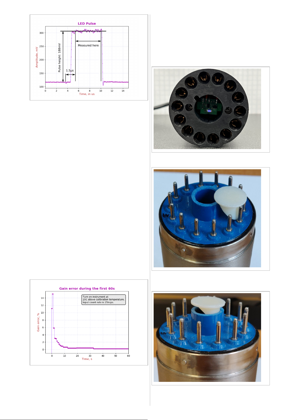
Adjusting the diffuser: First keep the LED off
and adjust the gain of the detector as desired.
Then, insert the diffuser, turn the LED on, set
sel_led=1 , trace_mode=0 and acquire a few
traces. You will see a rectangular LED pulse
with a width that can be controlled with the
led_width control. For now we are only
concerned about the pulse height.
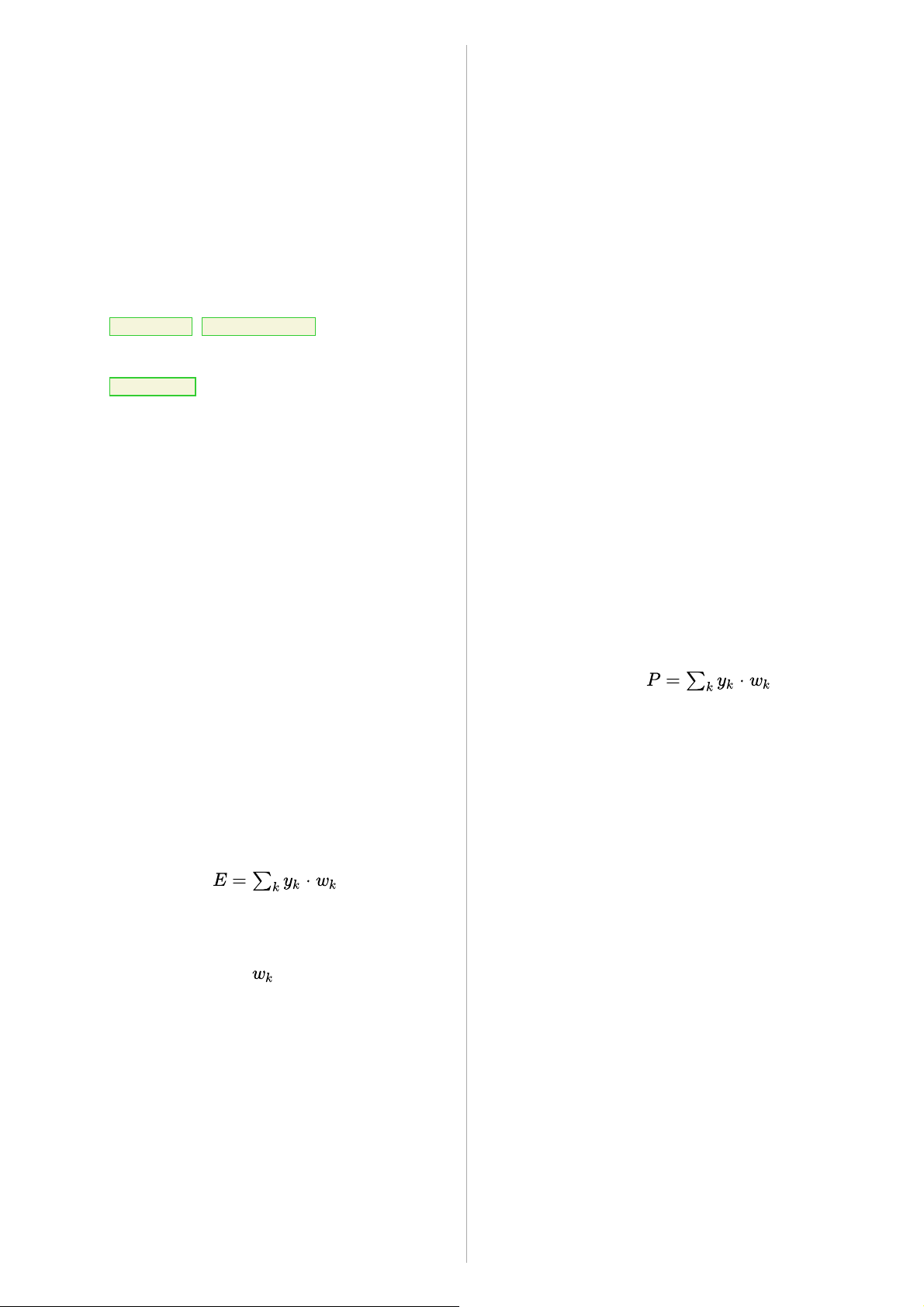
In the MCA the LED is placed off-center and
the light diffuser is asymmetric. Turning the
light diffuser changes the amount of LED light
transmitted into the PMT. You have to unplug
the PMT-3000 from the PMT in order to turn
the light diffuser. Note that you have to power
down the MCA before plugging and
unplugging. Never hot-plug the PMT-3000. It
would damage the device.
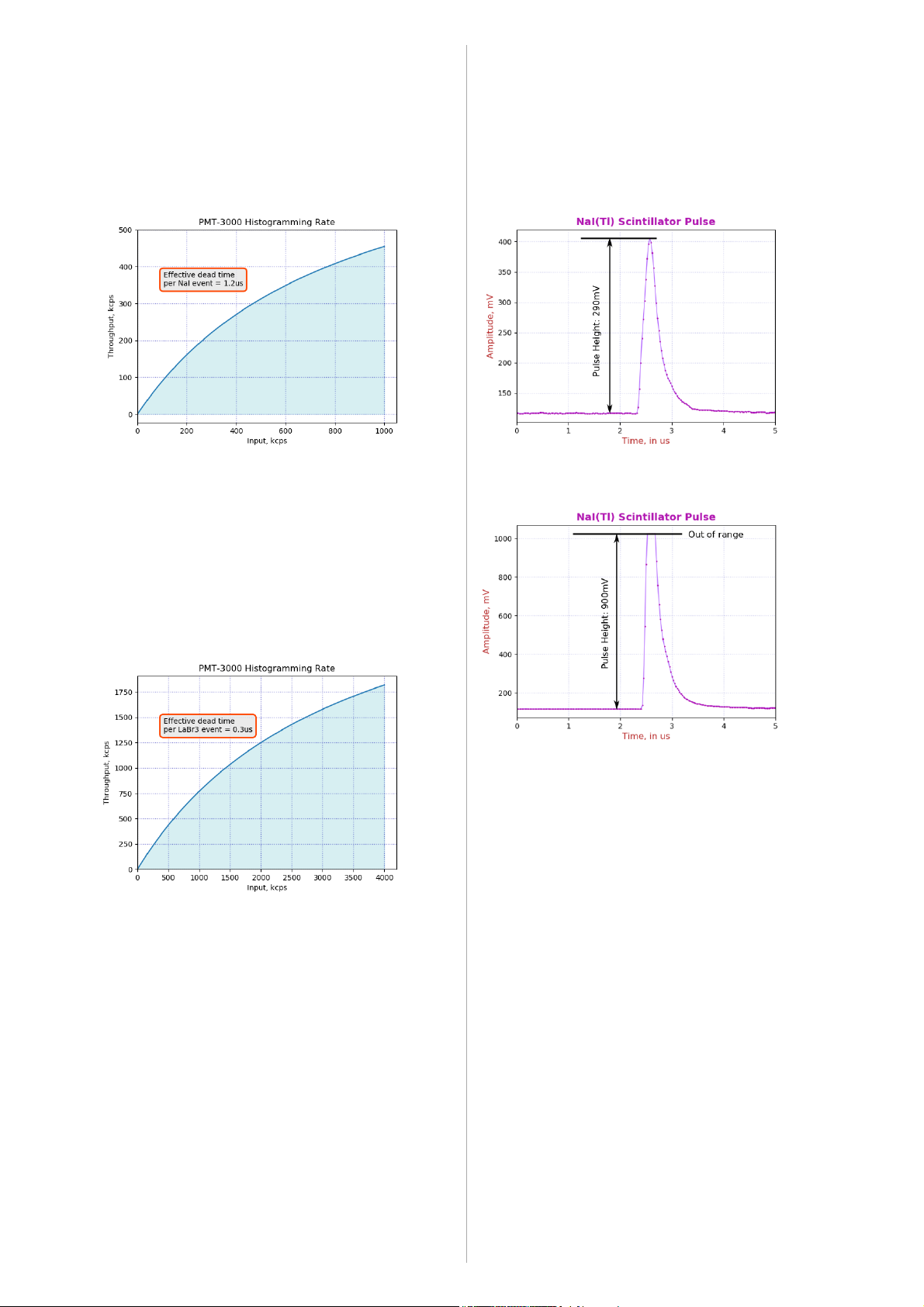
Aim for LED pulses of around 200mV ±50mV,
cf Fig. 5. Then glue the light diffuser into the
opening. For precise operation, the diffuser
must be securely glued in, otherwise it will
change its position during temperature cycles.
6. Summation Weights
Normally the MCA-3000 measures a pulse
energy by first subtracting the DC-baseline,
and then by summing all ADC samples over an
integration time. All ADC samples are weighed
equally. But the MCA-3000 offers a more fine-
tuned control:
Improve the performance of certain
scintillators. In some unusual scintillators the
energy resolution can be improved if the
summation weights are not all equal. One
example is SrI(Eu) where in big crystals the
self-absorption of its own scintillation light can
create significantly different pulse shapes for
the same amount of energy deposited in the
crystal; say for 662keV. The scintillator grower
may have a recommendation, or the user can
apply iterative or machine learning methods to
find an optimized set of summation weights.
Most often, however, summation weights will
be advantageously used to create powerful
pulse shape discrimination algorithms as
discussed in the section.
Within the FPGA, 1024 consecutive
summation weights are stored, which covers
integration times up to 8.53µs (@120MHz
ADC speed) or up to 51.2µs (@20MHz ADC
speed).
Ignore if not needed. By default all
summation weights are set to 32767. For the
purpose of energy measurement, the weights
are considered to be unsigned 16-bit integers,
with a range from 0 to 65535. Unless this
feature is used, users can completely ignore
this.
There is only one set of weights. When
psd_on=0, the weights are treated as uint16_t
and are used in the computation of the energy
sum. When psd_on=1, the weights are used for
the psd sum instead of the energy sum.
The software ships with a big examples
section, where the user can find short python
scripts to program custom weights into the
FPGA, and even store them in the ARM
processor's non-volatile memory.
7. Pulse Shape Discrimination
PSD is controlled by the user. Both MCA-
3000 support a very general, patented, pulse
shape discrimination method that gives the user
great control. The user can define 16-bit signed
weights to apply to each ADC sample in a
pulse after triggering. . For
each event the firmware classifies the event as
being type 0 or 1.
When PSD is turned on, the firmware separates
type 0 and 1 events into two separate halves
(2Kx32) of the available histogram memory.
Type 0 events are always histogrammed in the
lower half, while type-1 events are recorded in
the upper half. For both types of events there is
a separate event counter to measure count rates.
When PSD is turned on, the firmware separates
type 0 and 1 events into two separate halves
(2Kx32) of the available histogram memory.
Type 0 events are always histogrammed in the
lower half, while type-1 events are recorded in
the upper half. For both types of events there is
a separate event counter to measure count rates.
This feature is compatible with loss-less
histogram acquisition where the histogram is
split into two separate banks. In that case there
will be four 1Kx32 spectra.
See wxMCA/examples on how to program
the weights. Consult the examples folder of the
software to find code examples that write
summation weights to the FPGA of the MCA-
3000 and to the non-volatile memory of the
ARM processor.
E = ⋅
∑
k
y
k
w
k
w
k
P = ⋅
∑
k
y
k
w
k

Factory default: The factory default for the
weights is 32767, which is very nearly the
same as 1.0. When psd_on=0, the weights are
used for regular energy measurements, and
having all weights to be equal and near 1.0, is a
reasonable default.
When psd_on=1, the weights are used for pulse
shape discrimination (PSD). The default set
will not provide any PSD, and the user must
program a new set of weights. This is discussed
in detail below.
7.1 Where does the pulse begin?
In order to select the weights it is helpful to see
exactly where a pulse starts, ie to which ADC
sample the first weight is applied. To this end
set psd_on=1 and trace_mode=0 . Then
acquire a set of 10 pulses.
You will notice that the pulse peaks all occur at
the same time. The PMT-3000 issues its
internal trigger when the signal reaches its
peak. The weights summation starts at sample
0.
The distance between sample 0 and the pulse
peak is 12, 24 and 36 samples for ADC speeds
of 40MHz, 80MHz, and 120MHz, respectively.
7.2 A theoretical example
Here we consider a theoretical example to
explain how the PSD feature works. In the next
section we show a practical case.
Consider a phoswich detector in which beta-
particles create short pulses, and gamma-rays
create long pulses. Here we just consider a
much simplified version using two triangular
pules shapes. For simplicity, we also assume
that the trigger point is exactly at the start of
the rising edge.
Fig. 6:Pulse shape discrimination using summation weights.
Consider applying the weights wf to the fast
pulse. Because of the symmetry, the sum will
be zero. But the same wf weights applied to the
slow pulse will create P>0.
Similarly, applying the weights ws to the slow
pulse will result in P=0. But the same ws
weights applied to the fast pulse will create
P<0.
Hence, using a weight function that is between
wf and ws will map fast pulses to P<0 and slow
pulse to P≥0. The firmware uses 0 as the
decision point.
7.3 Weights format
Weights are signed 16-bit integers. When
pulse shape discrimination is turned on, the
weights are used as indicated in table 3. Since
most of the control and GUI software treats the
FPGA controls, and the summation weights as
unsigned 16-bit, consult the table below to
correctly encode the weights values.

PSD Weight uint16_t value
-1 32768, 0x8000
-0.5 49152, 0xC000
-0.25 57344, 0xE000
0 0, 0x0
0.25 8192, 0x2000
0.5 16384, 0x4000
1-1/32768 32767, 0x7FFF
Table 3: Encoding PSD weights as 2's complement
unsigned int 16. The largest possible positive value is
represented by 0x7FFF=32767. The most negative possible
value is represented by 32786=0x8000.
7.4 PSD controls
Set psd_on=1 to turn on pulse shape
discrimination. Set psd_sel=1 to histogram
the PSD sums used for the decision making,
instead of histgramming event energies.
You can control which type of pulse is
histogrammed in the low-bins of the
histogram memory. If weights start with a
block of negative values the condition P<0 will
select fast events and these will be
histogrammed in the lower part of the
histogram memory. A user can reverse this by
changing the sign of all weights. Now, P<0 will
select the slow pulses and the slow pulses will
be histogrammed in the lower part of the
memory.
Fast pulse and slow pulse count rates are
measured separately. The firmware uses two
extra sets of event counters. XCTR_0 counts
pulses for which P<0. XCTR_1 counts pulses
for which P≥0. Both extra counters and their
associated count rates are reported by the MCA
Data Server and are displayed in the GUI.
Note that XCTR_0 and XCTR_1 also accept
pulses arriving at their designated GPIO pins.
Feeding counting pulses into the GPIO pins of
XCTR_0 or XCTR_1 while using pulse shape
discrimination will lead to erroneous results.
7.5 PMT-3000 β/γ Example
For precision spectroscopy, the PMT-3000
slows down the scintillator pulses. When
using a β/γ phoswich made of a plastic
scintillator and a NaI-detector, the plastic
scintillator pulse is much faster than the NaI
light pulse, which makes pulse shape
discrimination an easy task in this case.
However, the user may decide to use a bigger
electronic gain to keep the PMT gain low and
reduce aging effects – while also using a
40MHz ADC for lowest power consumption.
Below we show the performance of such a
PVT/NaI phoswich detector.
Even small pulse shape differences can be
used. The phoswich was constructed using a
50mm×50mm NaI(Tl) crystal and a 3mm
plastic scintillator (PVT). The PMT-3000,
operating at 40MHz, was set to use the 3400Ω
gain setting to purposefully slow down the
electronic pulses.
Fig. 7: Average of 10000 beta and gamma traces, acquired
on a PMT-3000 at 40MHz digitization rate with a PVT/NaI
phoswich detector.
Observe in fig. 7 how the β-pulses (blue) are on
average slightly faster than the γ-pulses (red).
Their pulse width (fwhm) is about 250ns vs
500ns for the γ-pulses from the NaI. The
difference is clearly visible, but not very
pronounced. The grey pulse is the arithmetic
average between the two, and we will use it to
create the PSD filter.
Fig. 8: Average of 10000 beta and gamma traces, after
integrating the pulses starting at 0.
Observe in fig. 8 how the integrals of β-pulses
(blue) and γ-pulses (red) diverge strongly from
each other beyond 0.5µs. At 1.0µs the integrals
are markedly different for pulses that have the
same maximum pulse height. Using energy
integrals and , one can build a first PSD
equation . We want to choose
such that the dividing line shown in grey
E
0
E
1
P = − r ⋅
E
1
E
0
r

would map to zero . With that choice we
expect and .
In this example, we find that on the dividing
line, and , hence we
select in order to map the dividing
line to 0.
In the MCA-3000 the pulse integral is
approximated by sums over ADC samples. For
a 40MHz ADC, 0.50µs means 20 ADC
samples.
and
We can write the PSD sum
as , which here simply
becomes
We show this first iteration of the summation
weights in fig. 9
Fig. 9: Average of 10000 integrated beta and gamma traces,
now shown with a first estimate of PSD summation weights.
In practice, one finds that the performance can
be improved if the summation focuses on those
ADC samples where the signal to noise ratio is
big. For example, focusing the PSD sum on
those times where both the β- and the γ-pulses
are significantly greater than 0, helps to avoid
adding just noise to the sum without
accumulating meaningful information.
The MCA-3000 lets a developer tweak the
PSD summation weights to achieve the best
performance. In fig. 8 we show the result of a
practical tuning for the above-described
PVT/NaI phoswich. In this case, we had
adjusted the gain such that the maximum
measurable energy would be 1.6MeV and the
NaI-trigger threshold was set to 50keV. The
reasoning was that low-energy γ-rays (eg
30keV from Cs-137) will often be stopped in
the 3mm-thick plastic scintillator. This would
lead to many false beta counts, not because of
limits of MCA pulse shape analysis
capabilities, but because of the physics of γ-
rays.
Fig. 10: Average of 10000 integrated beta and gamma
traces, now shown with a tuned set of PSD summation
weights.
Inspecting fig. 10 shows the strength of the
approach. Instead of just comparing complete
energy sums, we can create partial sums at will,
as every weight can be set individually.
The MCA-3000 provides a tool for the
developer to judge the performance of the
pulse shape discrimination. In the
fpga_controls set psd_on=1 and psd_sel=1 .
In the Histogram panel set the number of
MCA bins to 4096, to see the entire spectrum.
Keep in mind the PSD decision sums are
centered around bin 2048 in this display.
With these settings you will see a 4K histogram
of the PSD sums. Events to the left of bin 2048
will fall in one class, and events in bins ≥ 2048
will fall into the other. The shape of the PSD
histogram on either side of the divide is not of
much interest. The only thing that counts is that
the right and left side of the spectrum are
separated by a clear gap.
Fig. 11 below shows an example. This one was
acquired using a weak Tl-204 source
encapsulated in 2mm of plastic in the presence
of natural γ background. In the PSD histogram
you can clearly see the two classes of events,
well separated by a gap around zero (ie the
middle of the 4K histogram).
P = 0
P ( β ) < 0 P ( γ ) > 0
= 10.6
E
0= 14.3
E
1
r = 1.351
=
E
0
∑
19
0
y
k
=
E
1
∑
39
20
y
k
P = − r ⋅
E
1
E
0
P =
∑
39
0
w
k
y
k
P = (1 − r ) +
∑
19
0
y
k
∑
39
20
y
k
w
k
E
0
w
k

Fig. 11: Pulse shape discrimination (PSD) histogram for Tl-
204 and background γ's using the PVT/NaI detector + PMT-
3000 and settings as described above. Here we set bin 2048
as 0 for clarity.
7.6 SiPM-3000 Example
In the SiPM-3000 PSD is limited to time
>150ns. In an SiPM-3000 the large capacitance
of a 3.4cm2 SiPM-array lengthens the pulse
width at the output of the input amplifier. At
the same time, the recharge time of a
Broadcom S4N66 SiPM is 150ns. Hence, pulse
shape discrimination is limited to times greater
than 150ns. Below we show that a PVT/NaI
phoswich detector will still perform well.
The fast scintillator can be much faster than
150ns. The phoswich was constructed using a
50mm×50mm NaI(Tl) crystal and a 3mm
plastic scintillator (PVT). The light pulse from
the PVT is only a few ns wide, but the SiPM-
array lengthens that to the recharge time of
150ns. On top of that, the input amplifier is
slowed down by the large capacitance of the
SiPM-array. As a result, we see the two
normalized and averaged pulse shapes; fast for
beta-particles being stopped in the PVT and
slow for gamma-rays interacting in the NaI.
Construction of the β/γ phoswich: The SiPM-
array is coupled to a dual-window NaI-
assembly. The SiPM-side is called the top.
Away from the SiPM, at the bottom, a plastic
scintillator is mounted against the NaI-
assembly. The plastic scintillator is at the
bottom side.
Construction of the summation weights:
Using summation weigthts is a very general
method to achieve pulse shape discrimination.
One way to arrive at a first useful set of
summation weights is to consider those regions
where the two types of traces are similar, and
where they are different.
In this case we apply a negative weight to the
region where the two traces are almost the
same. In the regions where the γ-ray pulse
values (from the NaI) are significantly bigger
than the blue β-pulse values, we apply a
positive weight. The value of the positive
weights is adjusted such that all βs map to <0
in the PSD histogram, and all γs map to >0 in
the PSD histogram.
The weights can then be varied to optimize the
PSD performance. Below we show the result
for the same PVT/NaI phoswich, but here used
with the SiPM-array instead of a PMT.
Fig. 12: Average of 10000 beta and gamma traces. In
addition we show the summation weights used to obtain good
β/γ separation.
PSD histogram An example β/γ PSD
histogram is shown in figure 13. Even with the
limited speed of the input amplifier in an
SiPM-3000, the beta/gamma separation is
nearly perfect.
Fig. 13: PSD histogram for the combination of a weak Sr-
90 source with a count rate equal to background γ's.

Item Performance
Sr-90 If detected, 95% are classified correctly.
Cs-137 <0.005% false betas; with Cs-137 above the
NaI top side.
Background ~0.2cps β
Settings Max γ-energy: 3.2MeV; trigger threshold at
50keV.
Table : Performance of the SiPM β/γ phoswich.
8. Analog
8.1 PMT-3000
The PMT-3000 combines a PMT operating
voltage supply and an MCA data acquisition
board with a structure as shown in the figure
below.
Fig. 14: The components of the PMT-3000.
The analog input of the PMT-3000 uses an I-to-
V converter with four programmable gain
resistors as shown in the figure below. A
gain_select of 0, 1, 2, 4, and 8 creates a
transimpedance of 100Ω, 430Ω, 1100Ω,
3400Ω, and 10100Ω, respectively.
Fig. 15: The input amplifier of the PMT-3000.
8.2 SiPM-3000
The SiPM-3000 combines a very low-noise
SiPM operating voltage supply and an MCA
data acquisition board with a structure as
shown in the figure below.
Fig. 16: The components of the SiPM-3000.
The analog input of the SiPM-3000 uses an I-
to-V converter with four programmable gain
resistors as shown in the figure below. A
gain_select of 0, 1, 2, 4, and 8 creates a
transimpedance of 5Ω, 20Ω, 55Ω, 155Ω, and
505Ω, respectively.
Fig. 17: The input amplifier of the SiPM-3000.
9. Mechanical and Pin Outs
9.1 8-Pin Connector
The PMT-3000 uses a Bulgin PX0447 mini-B
USB connector for power and USB
communication. Mating cables are the Bulgin
PX0441 (USB-A) and PX0442 (USB mini-A)
series cables. They come in lengths from 2m to
4.5m.
The PMT-3000 uses a Switchcraft EN3P8MPX
8-pin connector for GPIO and serial UART
communication. The mating connector is part
of the EN3C8 series.


Fig. 18: Pinout of the EN3P8 connector.
10. Product and Part Numbers
10.1 Product numbers
The PMT-3000 is part of a product series that
all contain an ARM M0+ 32-bit processor for
communication and slow control, such as gain
stabilization. In the -1000 series the MCA is
implemented by software in the ARM
processor. In the -3000 series the MCA is
implemented independently within an FPGA
for very high-speed operation. The -3000 series
also uses a waveform-digitizing ADC and
offers detailed pulse capture and real time pulse
shape discrimination.
Both types of devices are available for vacuum
photomultiplier tubes (PMT) and Si-
photomultipliers (SiPM). In both cases, the
device generates the operating voltage for the
photo-sensor from the incoming 5V.
P/N Sensor FPGA
PMT-3000 PMT Yes
SiPM-3000 SiPM Yes
Table : Part numbers.
10.2 USB-ID
On the USB bus devices are recognized by
their Vendor ID (VID), Product ID (PID) and
Serial Number (SN). The vendor ID for
Bridgeport Instruments is 0x1FA4. The Product
ID's are shown in the table below. Within a
product the serial number is fixed, unless BPI
makes a custom device that requires a non-
standard driver. Note that simple extensions,
such as adding a variable to the controls, does
not require a new driver.
The BPI software recognizes individual
devices by the unique serial number burnt into
each ARM processor. The device reports that
when the host reads arm_version. The serial
number communicated in response to USB
setup commands is fixed for each part, to avoid
that the host keeps adding every new device to
an ever longer list of devices requiring a
designated USB driver.
P/N PID SN
PMT-3000 0x0103 armMorpho0001
SiPM-3000 0x0203 sipmMorpho0001
Table : Product ID and USB bus serial numbers. The
vendor ID is always VID=0x1FA4.
10.3 Device serial numbers
Each ARM processor has an immutable 128-bit
unique serial number, which can be printed as a
32-character hexadecimal string. The MCA
Data Server always uses the complete 32-
character string to identify the device. Because
of space constraints, the serial number printed
onto the device is shortened to 8 hexadecimal
characters.
bpi_mca3k_um_v3p1.pdf© Bridgeport Instruments, LLC, 2021-03-11