10 Embedded Artists LPC4357 Guide 16 October 2013
Trace Examples
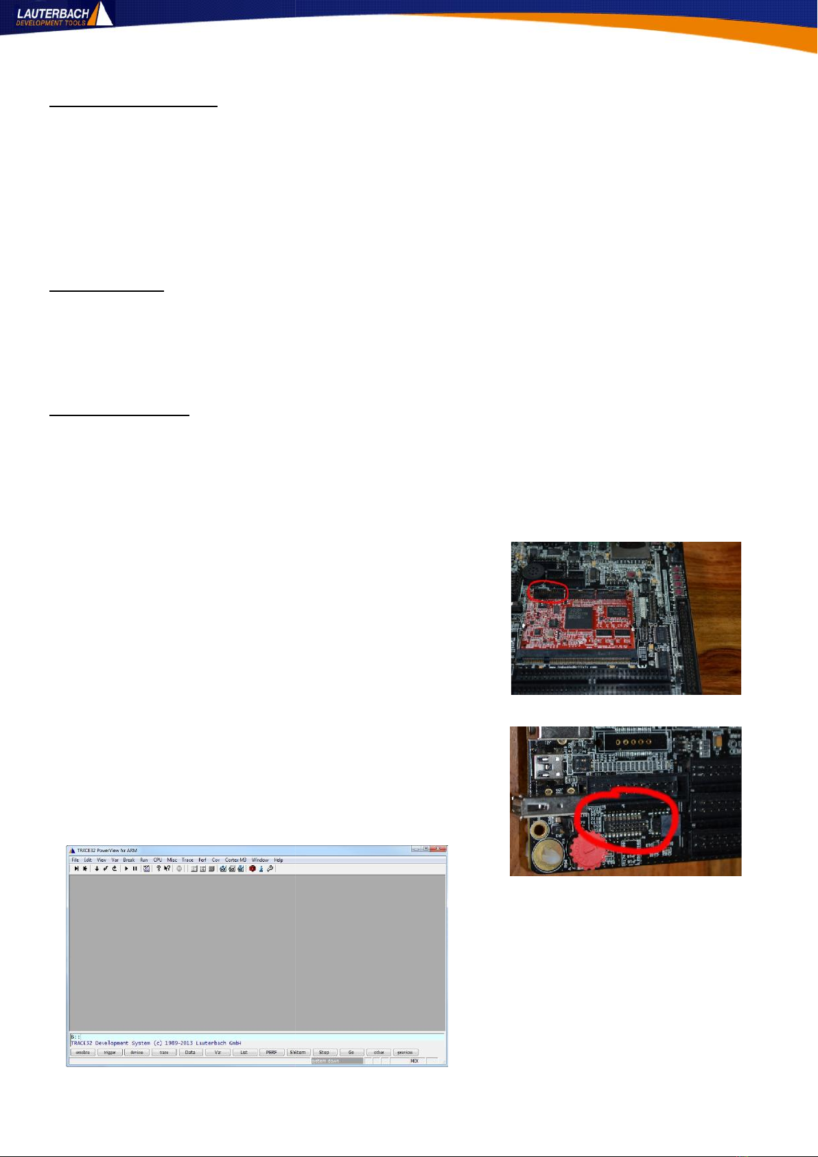
All of the previous tutorials have been using the JTAG or SWD interface. The next batch will look at using
the off-chip trace or ETM. The example scripts configure the trace port and pins but the board still needs to
be modified as described on page 4 so that the trace signals are available for the µTrace to capture.
Basic Trace Collection
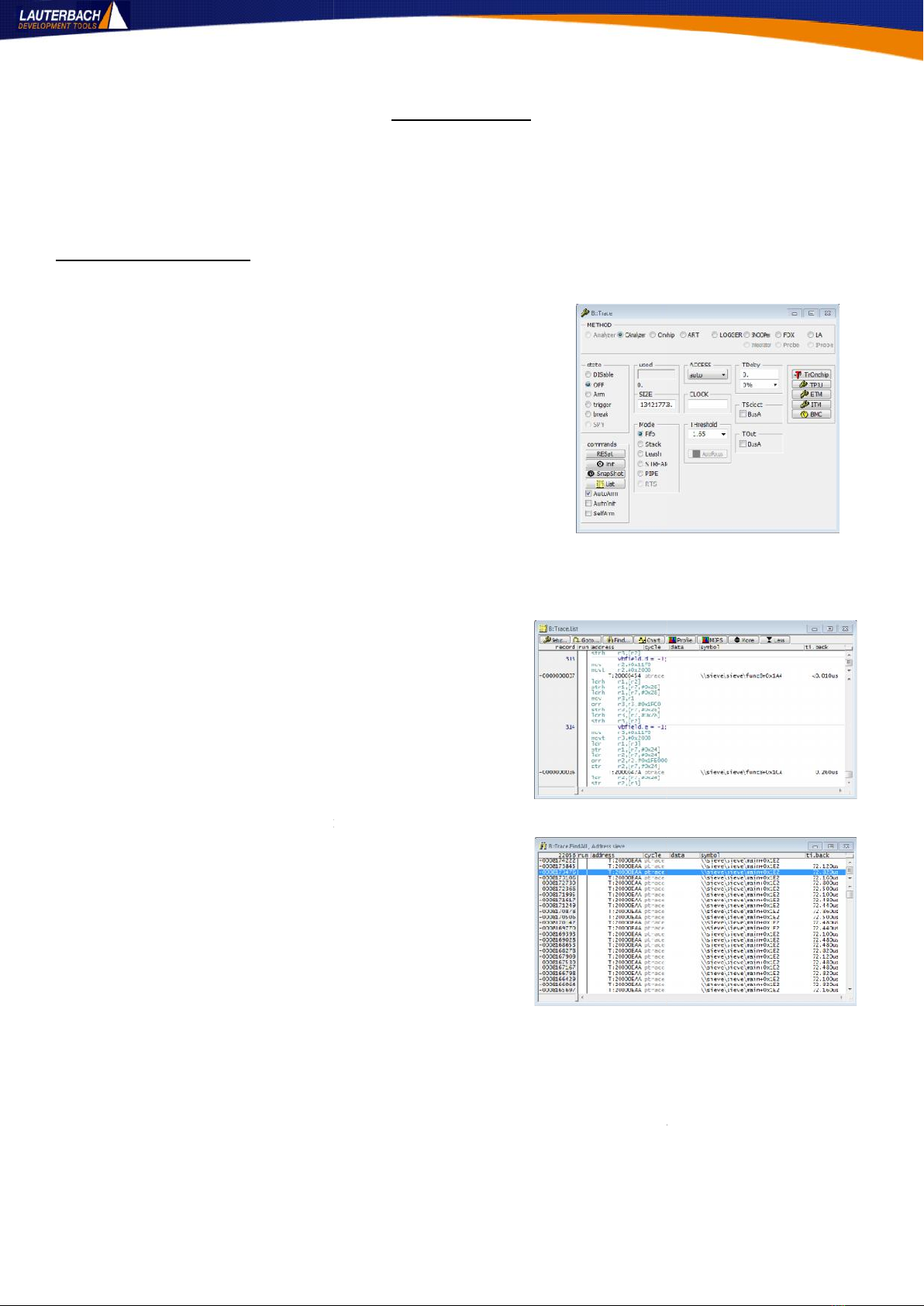
Select Configuration from the Trace menu. You should get a
window like that in figure T11. Make sure that the METHOD is
set to CAnalyzer and the state is set to OFF. Ensure that the
AutoArm box is ticked. This allows tracing to start and stop as
the target CPU starts and stops.
Start the target and let it run for a few seconds before
stopping it again. There should be a blue bar in the used box
to indicate the number of trace records captured. This should
number in the tens or hundreds of thousand for a few
seconds of run time. If it is less than a hundred or so you may
need to check the resistor positioning as there appears to be
no meaningful trace data.
Once you have some trace data captured, click the List
button and see the program flow information. The
window will look like figure T12. Click the More or Less
buttons to filter the amount of information displayed in
the window.
The trace data can be searched. Click the Find button
and enter the text “sieve” into the address/expression
box. Then click the Find All button. This will show a
window that looks like figure T13 with all occurrences of
calls to the function sieve in the trace buffer. Clicking on
any of these will cause the trace listing window to jump to
that point in the buffer so you can see the program flow
around that event.
The ti.back column in the search results window shows
the time between function calls. It should average out at
around 72.5us.
By default there is no data trace on the Cortex-M so data reads and writes will not be traced and cannot be
searched for. However, if the DWT on your device supports it you can use a data breakpoint (up to four of
them are allowed for in the Cortex-M specification but the actual number is core specific) to cause a data
trace event to be injected into the trace stream. Care should be taken when doing this as data trace
packets cannot be as easily compressed as the program flow trace packets and you may get an internal
trace FIFO overflow and some data will be lost.
Figure T11: Trace Configuration
Figure T12: Program flow trace
Figure T13: Search Results
10 Embedded Artists LPC4357 Guide 16 October 2013
Trace Examples
All of the previous tutorials have been using the JTAG or SWD interface. The next batch will look at using
the off-chip trace or ETM. The example scripts configure the trace port and pins but the board still needs to
be modified as described on page 4 so that the trace signals are available for the µTrace to capture.
Basic Trace Collection
Select Configuration from the Trace menu. You should get a
window like that in figure T11. Make sure that the METHOD is
set to CAnalyzer and the state is set to OFF. Ensure that the
AutoArm box is ticked. This allows tracing to start and stop as
the target CPU starts and stops.
Start the target and let it run for a few seconds before
stopping it again. There should be a blue bar in the used box
to indicate the number of trace records captured. This should
number in the tens or hundreds of thousand for a few
seconds of run time. If it is less than a hundred or so you may
need to check the resistor positioning as there appears to be
no meaningful trace data.
Once you have some trace data captured, click the List
button and see the program flow information. The
window will look like figure T12. Click the More or Less
buttons to filter the amount of information displayed in
the window.
The trace data can be searched. Click the Find button
and enter the text “sieve” into the address/expression
box. Then click the Find All button. This will show a
window that looks like figure T13 with all occurrences of
calls to the function sieve in the trace buffer. Clicking on
any of these will cause the trace listing window to jump to
that point in the buffer so you can see the program flow
around that event.
The ti.back column in the search results window shows
the time between function calls. It should average out at
around 72.5us.
By default there is no data trace on the Cortex-M so data reads and writes will not be traced and cannot be
searched for. However, if the DWT on your device supports it you can use a data breakpoint (up to four of
them are allowed for in the Cortex-M specification but the actual number is core specific) to cause a data
trace event to be injected into the trace stream. Care should be taken when doing this as data trace
packets cannot be as easily compressed as the program flow trace packets and you may get an internal
trace FIFO overflow and some data will be lost.
Figure T11: Trace Configuration
Figure T12: Program flow trace
Figure T13: Search Results