Schäfter+Kirchhoff SK22368GTOC-LA User manual

© 2018-12 E [email protected] www.SuKHamburg.com
Instruction Manual SK22368GTOC-LA shared_Titel_ML.indd
SK22368GTOC-LA
Color Line Scan Camera
3x 7456 pixels 4.7 x 4.7 µm², line frequency up to 5.13 kHz
Instruction Manual
SK22368GTOC-LA
3
2
Sample Configuration
1CCD line scan camera
SK22368GTOC-LA
mounted with
2Mounting bracket SK5105-L
3Clamping claws SK5101
4Focus adapter FA22R-45 (two-piece),
facilitates adjustment of any rotation angle
5Enlarging lens Apo-Rodagon N 4.0/80
5
4
1
400 500 700 800600
Wavelength (nm)
0
Responsitivity
(V/mJ/cm2)
100
0.0
1.0
400 500 600
Wavelength (nm)
Relative sensitvity
color
Color line scan camera (Triple-Line) with 3 x 7456 RGB pixels, 5.13 kHz maximum line rate,
small pixel size and short sensor length.

Instruction Manual SK22368GTOC-LA shared_Hinweise.indd
2
Instruction Manual SK22368GTOC-LA © 2018-12 E
How to Use this Instruction Manual
Electricity Warning
Assembly and initial operation of the line scan camera must be carried out under dry
conditions.
Do not operate the camera if you notice any condensation or moisture in order to avoid danger
of a short circuit or static discharge!
Risk of High Power Lighting
According to the application, laser or high power LED light sources might be used. These can
affect your eyesight temporarily or even cause permanent damage to the eyes or skin.
Do not look directly into the light beam!
Mechanics Warning
Ensure that the motion device and the scan way is free to move and that no obstacles are in
the way.
Do not place any part of the body in the way of moving parts!
Line scan cameras are mostly used in combination with a motion device such as a translation
stage, a conveyer or a rotational drive, as well as with high intensity light sources.
For assembly close down these devices whenever possible. Beyond that, please consider the
following warnings:
Safety Warnings
Please read the following sections of this Instruction Manual before unpacking, assembly or use
of the Line Camera System:
The safety warnings on this page
Introduction to the system, page 4
Installation and Setup, page 7
Keep this Instruction Manual in a safe place for future reference.
!

Instruction Manual SK22368GTOC-LA shared_Contents.indd
3
Instruction Manual SK22368GTOC-LA © 2018-12 E
Contents
How to Use this Instruction Manual 2
Safety Warnings 2
Contents 3
1 Introducing the SK22368GTOC-LA Line Scan Camera  ������������������������������������������ 4
1.1 Intended Purpose and Overview 4
1.2 System Setup at a Glance 5
1.3 Computer System Requirements 6
1.4 SK22368GTOC-LA Line Scan Camera - Specifications 6
2 Installation and Setup ������������������������������������������������������������������������������� 7
2.1 Mechanical Installation: Mounting Options and Dimensions 7
2.2 Electrical Installation: Connections and I/O Signals 8
2.3 GigE Connections and SkLineScan Software Installation 9
SkLineScan Installation 9
Network Driver Installation 9
SkLineScan Start-up 10
Camera Setup 10
Initial Function Test 10
3 Camera Control and Performing a Scan  �������������������������������������������������������� 12
3.1 Software: SkLineScan 12
Function Overview: SkLineScan Toolbar 12
Visualization of the Sensor Output 13
3.2 Adjustments for Optimum Scan Results 14
Lens Focussing 14
Sensor Alignment 15
Gain/Offset Adjustment 15
White Balance and Shading Correction 16
Optimum brightness adjustment, Integration Time 19
Synchronization of the Image Acquisition with the Feed Rate of the Object 20
Synchronization Modes 21
RGB Sensors: 2D Imaging and Pixel Allocation 23
4 Advanced Camera Control Functions  ����������������������������������������������������������� 24
4.1 Camera Control by Commands 24
Set Commands 24
Request Commands 25
4.2 Advanced Synchronization Control 26
Advanced Trigger Functions and Sync Control Register (SCR) Settings 26
Example Timing Diagrams 27
5 Sensor Information �������������������������������������������������������������������������������� 28
Glossary 32
CE-Conformity 35
Warranty 35
Accessories 36

Introducing the SK22368GTOC-LA Line Scan Camera
Instruction Manual SK22368GTOC-LA shared_Introduction_GigE_ML.indd
4
Instruction Manual SK22368GTOC-LA © 2018-11 E
The SK line scan camera series is designed for a wide
range of vision and inspection applications in both
industrial and scientific environments. The GigE series
camera SK22368GTOC-LA uses the Gigabit Ethernet
communication protocol, enabling fast image transfer
using low cost standard cables up to 100 m in length. The
Gigabit Ethernet interface makes the line scan camera
highly scalable to faster Ethernet speeds, distinguishing
it with high performance and total flexibility.
All of the GigE cameras from Schäfter+Kirchhoff are
externally synchronizable and no grabber board is
needed as signal preprocessing is performed inside the
camera and does not impinge on CPU use.
Additional features include:
• customer-specific I/O signals in addition to the video
signal
• specialpreprocessingalgorithmscanbeimplemented
in the camera
• consistent attribution of camera IDs in multi-camera
operations
• SDK from Schäfter+Kirchhoff with the SkLineScan
operating program, libraries and examples.
1 Introducing the SK22368GTOC-LA Line Scan Camera
1.1 Intended Purpose and Overview
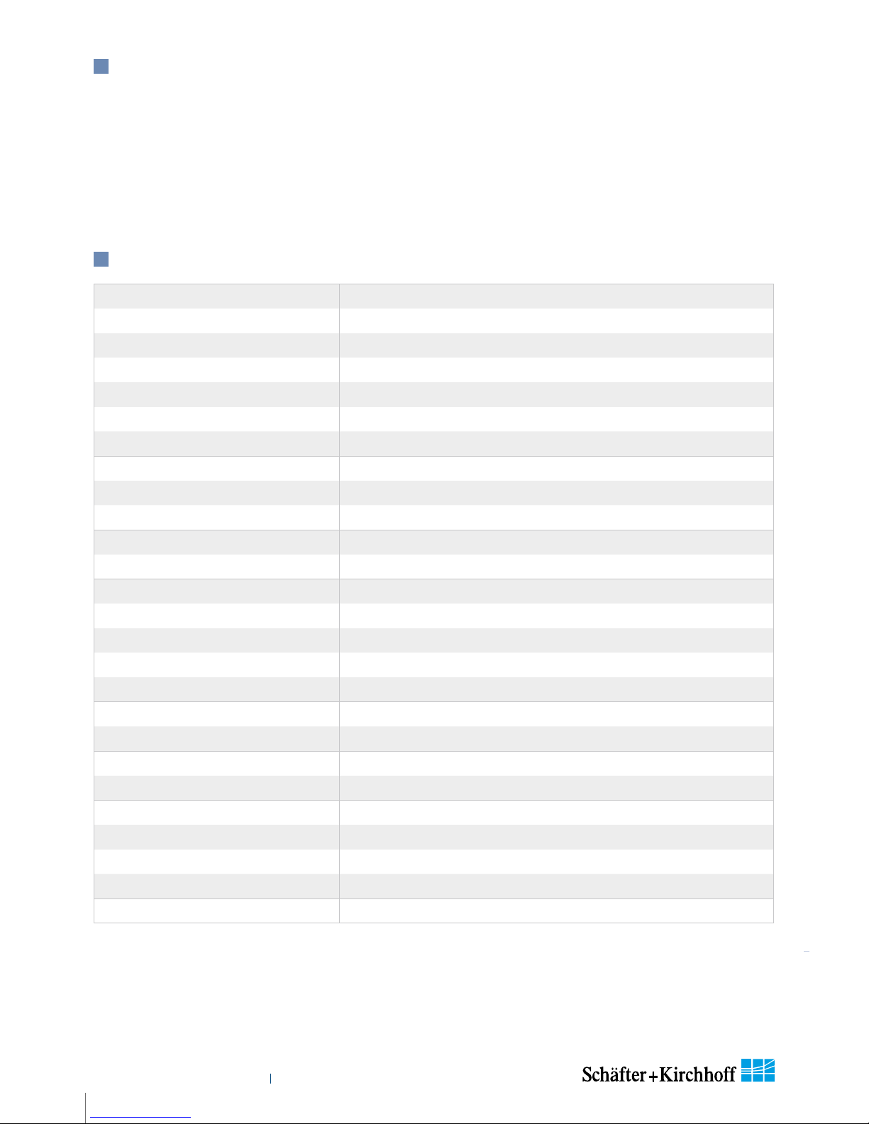
Features
Shading Correction X
Programmable Lookup Table X
Thresholding X
Window Function (ROI) X
Line Trigger, Frame Trigger X
Frame Trigger Delay X
Threshold Trigger X
Advanced Synchonization Ctrl. X
Integration Control for R, G, B X
Decoupling of line frequency X
Extra signals for diagnosis X
Data cable length 100 m
Windows SK91GigE-WIN SDK
LabVIEW SK91GigE-LV VI Library
Linux -
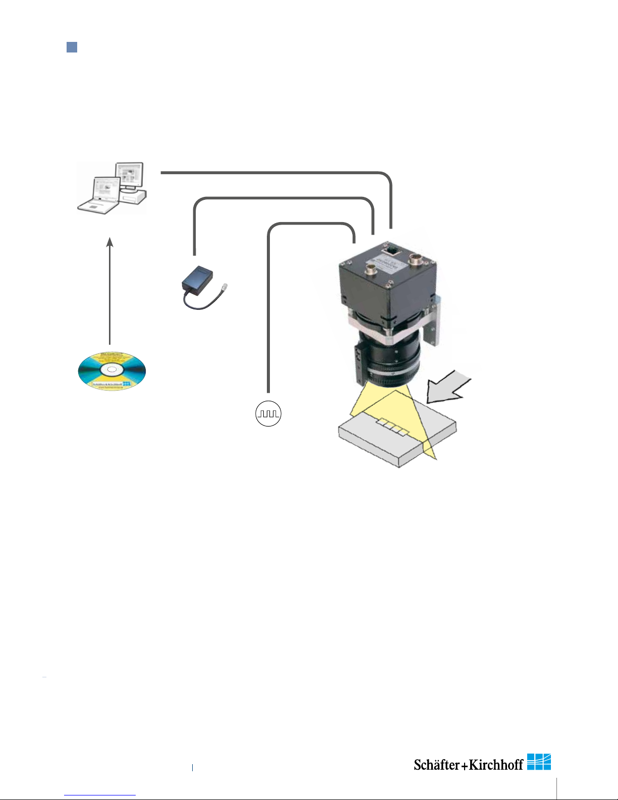
The camera can be connected to a computer either via
the GigE socket directly or through a Gigabit Ethernet
switch.
Once the camera driver and the SkLineScan® program
have been loaded from the SK91GigE-WIN CD then the
camera can be parameterized. The parameters, such
as integration time, synchronization mode or shading
correction, are permanently stored in the camera even
after a power-down or disconnection from the PC.
The oscilloscope display in the SkLineScan® program
can be used to adjust the focus and aperture settings, for
evaluating field-flattening of the lens and for orientation
of the illumination and the sensor, see 3 Camera Control
and Performing a Scan (p. 12).CCD line scan camera
2Power supply
3Illumination
Software, SDKs and eBus
driver
GigE switch
14
5
PC or
Notebook
with GigE
GigE interface for transmission
of video and control data over
distances up to 100 m
421
3
Advanced
preprocessing
Fixed camera
IDs for multi-
camera systems
Application:
Parallel
acquisition
using a
GigE switch
4
2
1
5

Introducing the SK22368GTOC-LA Line Scan Camera
Instruction Manual SK22368GTOC-LA shared_Introduction_GigE_ML.indd
5
Instruction Manual SK22368GTOC-LA © 2018-11 E
1.2 System Setup at a Glance
red: SK22368GTOC-LA scope of delivery
blue: accessories for minimum system configuration
black: optional accessories
For accessory order details see Accessories (p. 36).
Motion unit
with
encoder
Synchronization cable
Power supply cable
Gigabit Ethernet cable
Computer
Power supply
unit
Schäfter+Kirchho
SkLineScan®adjustment
and control software
Schäfter+Kirchhoff
Software Development Kit
Schäfter+Kirchhoff
VI library for LabVIEW®
Line scan camera
Clamping claw
Mounting bracket
Optics (e. g. lens,
focus adapter, tube
extension ring)

Sensor category CCD Color Sensor
Sensor type TCD2716DG
Pixel number 3x 7456
Pixel size (width x height) 4.7 x 4.7 µm2
Pixel spacing 4.7 µm
Line spacing, line sequence 18.8 µm, red (R) - green (G) - blue (B)
Active sensor length 35.04 mm
Anti-blooming -
Integration control -
Shading correction x
Line synchronization modes Line Sync, Line Start, Exposure Start
Frame synchronization x
Pixel frequency 120 / 60 MHz
Maximum line frequency 5.13 kHz
Integration time 0.195 ... 20 ms
Dynamic range 1:1000 (rms)
Spectral range 350 ... 700 nm
Video signal color 3*8 Bit digital
Interface GigaBit Ethernet
Voltage +5V, +15V
Power consumption 5.5 W (= 5V · 850mA + 15V · 80mA)
Casing 65 mm x 65 mm x 72.4 mm (Case type BG3)
Objective mount M45x0.75
Flange focal length 19.5 mm
Weight 0.3 kg
Operating temperature +5 ... +45°C
Introduction
Instruction Manual SK22368GTOC-LA shared_SystemRequirements_Specs_ML.indd
6
Instruction Manual SK22368GTOC-LA © 2018-12 E
1.3 Computer System Requirements
1.4 SK22368GTOC-LA Line Scan Camera - Specifications
Introduction
• Intel Pentium Dual Core or AMD equivalent
• RAM min. 4 GB, depending on size of acquired
images
• High-performance video card, PCIe bus
• Operating Systems:
Windows 7 / 8.1 / 10 (64 or 32-bit) or
Linux kernel 3.13 or higher
• CD/DVD drive for software installation.
Network Adapter:
• Any Gigabit Ethernet network adapter as a card
or on the motherboard is suitable. For the best
performance, a network interface card (NIC) with
Intel PRO/1000 chip is recommended.
• PCIe adapters outperform PCI adapters.
• Network adapters that support Jumbo Frames
outperform adapters with fixed packet-size frames.

Installation and Setup
Instruction Manual SK22368GTOC-LA shared_Installation-Mechanic_Axx-BGx_ML.indd
7
Instruction Manual SK22368GTOC-LA © 2018-12 E
2 Installation and Setup
2.1 Mechanical Installation: Mounting Options and Dimensions
Casing type BG3
Mounting Options
• The best fixing point of the camera is the collar for
the mounting bracket SK5105-L (available as an
accessory).
• Four threaded holes M3x 6.5 mm provide further
options for customized brackets.
• The length and weight of the optics might be beyond
the capability of the standard mounting bracket
SK5105-L. For this purpose, a second mounting
bracket type SK5105-2L to hold the tube extension
ring(s) is more appropriate.
Optics Handling
• If the camera and the optics are ordered as a kit,
the components are pre-assembled and shipped
as one unit. Keep the protective cap on the lens
until the mechanical installation is finished.
• If you must expose the sensor or lens surface,
ensure the environment is as dust-free as possible.
• Gently blow off loose particles using clean
compressed air.
• The sensor and lens surfaces can be cleaned with
a soft tissue moistened with water or a water-based
glass cleaner.
Mounting bracket SK5105-L
Mounting system SK5105-2L
for cameras with a tube
extension > 52 mm
Clamping set SK5101
Set of 4 pcs. clamping claws
incl. screws
66
10 10
36
M3 Ø3.3
6
50.3
41.7
Ø 47.5
50
20
16.5
3.5
6.5
Ø4.3
15 M4
1/4’’ 20G
40
63
70
6
36
Ø 47.5
70
3.5 31.5
25
10
3.5
70
63
40
1/4’’20G
M4
Ø4.3
Hex socket head screw
DIN 912–M3x12
Clamping claw
65
72.4
Ø65
Ø47.5
Pixel 1
M3 (4x)
depth 6.5 mm
65
M45x0.75
58
41.7
BG3 Lens mount: M45x0.75
Seat for bracket: Ø47.5 mm
Flange focal length: FFL = 19.5 mm
CCD-Sensor
2.5 6
4 25.1 FFL
12.7
50/M3/4x90°

1Power +5 V, +15 V Hirose series 10A, male 6-pin
Total power:
5.5 W (= 5V · 850mA + 15V · 80mA)
Pin Signal Pin Signal
1+15 V 4+5 V
2+15 V 5GND
3+5 V 6GND
2
1
3
4
5
6
7
8
9
10
1112
2
1
3
4
5
6
Power Cable SK9015.xMF
Use this cable to feed external supply voltage into socket 1.
Connectors:
Hirose plug HR10A, female 6pin (camera side)
Lumberg SV60, male 6-pin connector (for supply voltage)
Length 1.5 m (standard) or 0.2 m
Power Supply Unit PS051515
Input: 100-240 VAC, 0.8 A, 50/60 Hz, IEC 320 C14 coupler
(for IEC C13 power cord)
Output: +5V DC, 2.5 A / +15 V DC, 0.5 A / -15 V DC, 0.3 A
Cable length 1 m, with Lumberg connector KV60,
female 6-pin
(for power cable SK9015.x or SK9016.x)
3
1
2
Installation and Setup
Instruction Manual SK22368GTOC-LA shared_Installation-Electric_GigE+V_ML.indd
8
Instruction Manual SK22368GTOC-LA © 2018-12 E
2.2 Electrical Installation: Connections and I/O Signals
External Synchronization Cable SK9024.x
Use this cable to feed external synchronization
signals into socket 2.
Connectors:
Hirose plug HR10A, female 12pin (camera side)
Phoenix 6 pin connector incl. terminal block (for
synchronization signals)
Length 3 m or 5 m. Other lengths on request.
Network Cable CAT6.x
For connecting socket 3with the PC Ethernet
interface. Both ends with RJ45 connectors.
• For the SK22368GTOC-LA line scan camera-data transfer and camera control is provded by the Gigabit
Ethernet interface 3. Use a CAT6 twisted-pair cable to connect the camera to a PC; the maximum cable
length is 100 m.
• The operating power must be supplied by an external source using socket 1
• If you want to operate the camera in FREE RUN trigger mode, the connections are complete with the CAT6
Ethernet cable and the connection to an external power supply.
• For any kind of synchronized operation, the external trigger signal(s) must be wired to socket 2as well. A
frame-synchronization signal and two separate line-synchronization signals can be handled. The various
trigger modes are described fully in section Synchronization of the Image Acquisition with the Feed Rate
of the Object (p. 20)
2
1
3
4
5
6
7
8
9
10
1112 2
1
3
4
5
6
Pin Signal *)
1GND
8FrameSync IN
10 LineSync A IN
6LineSync B IN
2I/O Connector Hirose series 10A, male 12-pin
*) Signal Specification
(TTL) Max. input frequency 16.5 MHz
Input voltage,
absolute max. range
min -0.5 V
max 7.0 V
Input voltage max. low 0.99 V
Input voltage min. high 2.31 V
Input current 10 µA
Installation and Setup
3Data
RJ-45 connector for Gigabit Ethernet cable
Status indicators
Network connection speed Network activity
off no connection,
10 Mbyte/s connection, or
100 Mbyte/s connection
on 1 Gbyte/s connection
off no connection
on connected
flash
light
data is being
transmitted or
received
Accessories (see also Acessories (p. 32):

Installation and Setup
9
Instruction Manual SK22368GTOC-LA shared_Installation-Software_GigE.indd
Instruction Manual SK22368GTOC-LA © 2018-12 E
2.3 GigE Connections and SkLineScan Software Installation
SkLineScan Installation
Prior to the installation, power on the PC (not the camera) and unpack the downloaded zip-file to a temporary
folder. Alternatively, if your installation medium is a CD, insert the disk to the drive.
The autostart function may launch the setup program automatically from CD. Otherwise, look for one of these
installation files:
SkLineScan-GigE-Win_x64.msi SK91GigE-Win_x64.msi
SkLineScan-GigE-Win_x86.msi SK91GigE-Win_x86.msi
Then start the applicable installation file manually. This will set up the Schäfter + Kirchhoff SkLineScan camera
control and adjustment tool as well as the Pleora Network Driver Installation Tool.
Network Driver Installation
a) High Performance Driver for Intel PRO/1000 Chip
• If the line scan camera is connected to a network interface card (NIC) with Intel PRO/1000 chip, then
install the "High Performance IP Device Driver". This is the recommended system configuration for
optimum performance. Under Windows10 proceed as described
in the section "Standard GigE Network Adapters" below.
Open the program menue Aand start the network driver installation
manually:
• For 64-bit operating systems choose
“Driver Installation x64".
• For 32-bit systems (Windows 7 32-bit, XP) use
“Driver Installation x86”.
The eBUS driver installation tool window Bwill show up to list the
available network adapters and the currently installed network drivers in the system.
B
Plug in the CAT6 network cable to the camera and switch on the power supply. Then restart the system and check
the driver installation with the driver installation tool C.
C
The High-Performance driver is installed, further network adjustments are not required.
Step 1: Install SkLineScan
Step 2: If the Gigabit network interface controller (NIC)
has an INTEL PRO/1000 chip then install the High
Performance Driver
Step 3: Plug in the CAT6 network cable to the camera
and switch on the power supply.
Step 4: Check the network connection.
Step 5: Start the SkLineScan program.
Installation and Setup
This section is a quick reference for installing the SkLineScan adjustment and configuration software and to set
up the Gigabit Ethernet network adapter. SkLineScan and the SkLineScan manual is provided for download on
the Schäfter + Kirchhoff website under http://www.sukhamburg.com/support.html. It is also part of the fee-based
software development kit SK91GigE-WIN.
A
Start Driver Installation Tool
from Start Menue

Installation and Setup
Instruction Manual SK22368GTOC-LA shared_Installation-Software_GigE.indd
10
Instruction Manual SK22368GTOC-LA © 2018-12 E
b) Standard GigE Network Adapters
• For non-Intel PRO/1000 network adapters or
for Intel PRO/1000 network adapters under
Windows 10 install the driver recommended by
the manufacturer.
!This kind of GigE network adapters do require
additional setup. These settings should be
optimized during installation in the Advanced
Properties tab Dof the Network Adapter:
Jumbo Frames 9014 Bytes
Receive Descriptors 2048
Interrupt Moderation Rate extreme
Energy Efficient Ethernet OFF
LAN adapters for GigE cameras that do not
work with the High Performance Driver must
use a fixed IP address, e.g. 192.168.0.99.
SkLineScan Start-up
• Start SkLineScan. A start-up dialog box pops up
and displays the connected cameras that have
been automatically detected.
Camera Setup
Use the Setup dialog for
• activating/deactivating a connected
GigE camera (activated device is
ticked)
• changing the IP address
• changing the pixel frequency
• setting the bit depth of the video
signal to 8 or 12-bit.
The MAC addresses are displayed for identification of each camera with the defined CamID (0, 1, …). This is
useful when several cameras with the same name are connected.
SkLineScan Setup dialog
Network Controller Properties: Note, the terms
can differ depending on the installed Ethernet
card and driver.
D
Desktop Icon
Initial Function Test
• Quit the SkLineScan startup dialog
box.
• Select "OK" in the SkLineScan
start-up dialog.
The Signal Window showing the current
brightness versus the pixel number
indicates the correct installation.

Instruction Manual SK22368GTOC-LA shared_blank.indd
11
Instruction Manual SK22368GTOC-LA © 2018-12 E

Camera Control and Performing a Scan
Instruction Manual SK22368GTOC-LA shared_CameraControl(1)_SkLineScan_ML.indd
12
Instruction Manual SK22368GTOC-LA © 2018-12 E
3 Camera Control and Performing a Scan
3.1 Software: SkLineScan
This section is a brief introduction to the SkLineScan adjustment and configuration software. A more detailed
description is provided in the separate SkLineScan manual. The pdf is included in the SkLineScan installation
package or is available for download from the Schäfter + Kirchhoff website under http://www.sukhamburg.com/
supporte.html.
Detailed instructions on how to obtain optimal image data and use the data with the Schäfter+Kirchhoff
software package can be found in the SkLineScan Software Manual.
The most common functions of the line scan camera can be controlled by menu items and dialog boxes.
In the "Camera Gain / Offset Control" dialog there is a command line for entering further control commands.
Click on the desktop icon to start the SkLineScan
program.
The SkLineScan program recognizes the connected line
scan cameras automatically. The identified cameras are
shown in the start-up dialog A.
If the SK22368GTOC-LA camera is identified correctly,
confirm with "OK". The "Signal window" graphicaly
showing the intensity signals of the sensor pixels (oscil-
loscope display) will open. It is responsive in real-time
and the zoom function can be used to highlight an area
of interest. The oscilloscope display is ideally suited
for parameterizing the camera, for evaluating object
illumination, for focussing the image or for aligning the
line scan camera correctly.
Function Overview: SkLineScan Toolbar
Platzhalter für Grafiken in anderen Ebenen
New line scan. All open "Signal window" windows will be closed. [F2]
"Camera Control" dialog for parameter settings: integration time, line frequency, synchronization
mode, thresholding
Zooming in and out
New line scan. "Area Scan" windows will be closed, "Signal window" windows will remain open. [F2]
Threshold mode in new binary signal window.
"Shading Correction" dialog to adjust the white balance [Alt+ s]
"Gain/Offset Control" dialog, also for commands input [Shif+F4]
New area scan
SkLineScan: Toolbar
SkLineScan: Start-up dialog
A

Bedienung der Kamera und Durchführung eines Scans
Instruction Manual SK22368GTOC-LA shared_CameraControl(1)_SkLineScan_ML.indd
13
Instruction Manual SK22368GTOC-LA © 2018-12 E
Visualization of the Sensor Output
• Signal Window / Oscilloscope Display
The signal window plots the digitalized brightness profile as signal intensity (y-axis) versus the sensor length (x-axis)
at a high refresh rate. The scaling of the y-axis depends on the resolution of the A/D converter: The scale range is
from 0 to 255 for 8-bits and from 0 to 4095 for 12-bits. The scaling of the x-axis corresponds with the number of
pixels in the line sensor.
Platzhalter für Grafiken in anderen Ebenen
• Zoom Function
With a high number of sensor pixels, details are lost due to the limited number of display pixels. With the zoom
function you select a part of the sensor for the detailed display. The possible magnification ranges up to the repre-
sentation of the intensity signal of individual pixels.
• Window Split Function
The signal window can be divided horizontally into two areas. Use the slider Bat the top of the vertical scroll bar.
If you then use the zoom function in one frame, the selected section in the other frame will be highlighted in yellow.
Platzhalter für Grafiken in anderen Ebenen
Line scan in Signal
Window: brightness
vs. pixel number
B
Line scan in split
signal window: The
upper frame shows
an enlarged section
of the lower frame.

Camera Control and Performing a Scan
Instruction Manual SK22368GTOC-LA shared_CameraControl(2)_Adjustments-1_ML.indd
14
Instruction Manual SK22368GTOC-LA © 2018-12 E
Camera Control and Performing a Scan
3.2 Adjustments for Optimum Scan Results
•Lens focussing
•Sensor alignment
•Gain/Offset
•Shading correction
•Integration time
•Synchronization of the sensor exposure
and the object surface velocity, trigger
mode options.
Prior to a scan, the following adjustments and parameter settings should be considered for optimum
scan signals:
Start with the signal window / oscilloscope display. Any changes in the optical system or camera parameters
are displayed in real-time when using an open dialog box.
Lens Focussing
The real time Signal Window facilitates the effective focussing of the line scan camera system, even for
two-dimensional measurement tasks. For determining the correct focus, the edge steepness at dark-bright transi-
tions and the modulation of the line scan signal are the most important factors.
Adjust the focus with the aperture fully open to limit the depth of field and enhance the effects of changing the
working distance.
If the sensor is overloaded when the aperture is fully open, the easiest way to reduce the signal amplitude is to
shorten the integration time, as described in section Optimum brightness adjustment, Integration Time (p.
19).
Out-of-focus:
• Low edge steepness
• Signal peaks are blurred
• High spatial frequencies with low modulation depth
Optimum focus:
• Dark-bright transitions with steep edges
• Large modulation in the signal peaks
• High spatial frequencies with high modulation depth
steep edges
high modulation
depth
low modulation depth
low edge steepness

Camera Control and Performing a Scan
15
Instruction Manual SK22368GTOC-LA shared_CameraControl(2)_Adjustments-1_ML.indd
Instruction Manual SK22368GTOC-LA © 2018-12 E
Sensor Alignment
If you are using a linear light source, check the alignment of the light source and sensor before shading correction,
as rotating the line sensor will result in asymmetric vignetting.
Sensor and line lighting slightly twisted in
relation to each other, asymmetric vignetting
Sensor and line lighting aligned in parallel,
symmetric vignetting
Gain/Offset Adjustment
The cameras are supplied with factory-set gain/offset. Open the "Gain/Offset Control" dialog to adjust these
settings.
Platzhalter für Grafik und Text in anderen Ebenen
Adjustment principle
1. Offset
To adjust the zero baseline of the video signal, totally
block the incident light and enter "00" (volts) for
channel 1.
For a two- or multi-channel sensor, minimize any diffe-
rences between the channels by adjusting the other
Offset sliders.
A slight signal noise should be visible in the zero
baseline.
2. Gain
Illuminate the sensor with a slight overexposure in order
to identify the maximum clipping. Use the Gain slider
"1" to adjust the maximum output voltage.
For a two- or multi-channel sensor, minimize any diffe-
rences between the channels by adjusting the other
Gain sliders.
For the full 8-bit resolution of the camera, the maximum
output voltage is set to 255 and for 12-bit is set to
4095.
Offset
and gain
adjustment
for more than
one gain/
offset channel
2. Adjust the gain of channel 1.
Minimize the difference
between the channels with
the other gain controls.
1. Adjust the zero level of
channel 1. Minimize the
difference between the
channels using the other
Offset controls.
The gain/offset dialog contains up to 6 sliders for altering gain and offset. The number of active sliders depends
on the individual number of adjustable gain/offset channels of the camera. If "Coupled Gain Channels" is checked,
all channels are set synchronously with one slider.
Enter commands for advanced software functions in the 'Camera Control' field (see page 14).
Gain/Offset
Control dialog

Camera Control and Performing a Scan
Instruction Manual SK22368GTOC-LA shared_CameraControl(2b)_ShadingCorrection_col.indd
16
Instruction Manual SK22368GTOC-LA © 2018-04 E
Shading Correction compensates for non-uniform illumination and lens vignetting, as well as any differences in
pixel sensitivity. The signal from a white homogeneous background is obtained and used as a reference to correct
each pixel of the sensor with an individual factor. The result is a leveled signal along the full sensor length. A
shading correction with a balanced RGB sensitivity ensures a natural color reading. The reference signal is stored
in the Shading Correction Memory (SCM) of the camera and subsequent scans are normalized using the scale
factors from this white reference.
Step 1: White Balancing
• Use a homogeneous white object, e.g. a white sheet of paper, to acquire the RGB line signals.
Color line signal with separated RGB curves
White Balancing by Gain Adjustment
• Open the "Gain/Offset Control" dialog. Use the gain sliders to adjust all three curves to the same level. Some
camera models provide two gain/offset channels - thus two sliders - per color.
"Gain/Offset Control" Dialog
Camera Control and Performing a Scan
White Balance and Shading Correction

Camera Control and Performing a Scan
17
Instruction Manual SK22368GTOC-LA shared_CameraControl(2b)_ShadingCorrection_col.indd
Instruction Manual SK22368GTOC-LA © 2018-04 E
White Balancing by Individual Integration Time Control
In some circumstances, it is not possible to adjust the white
balance using the gain setting because of:
• dynamic limitations from a very intensive or weak illumination,
• undesired changes in noise level.
For such situations, an individual adjustment of integration times for the Red, Green, and Blue channels is
available, for a general description of the integration time adjustment, see section Optimum brightness
adjustment, Integration Time (p. 19).
Check that the weakest color signal is higher
than about 70%. If necessary, adjust the
line frequency or the illumination intensity
accordingly.
Tick the box "Decoupling LF" Ain the "Camera
Control" dialog.
Reduce the integration times for the two color
channels with the higher signals in order to align
the Red, Green and Blue channels to the same
level.
The Red channel is adjusted using the slider
"Exposure Time". B
For the Green and Blue channels, enter the
exposure time into the respective boxes. C
Color line signal with the Red signal adjusted to that of the Blue channel; the Green channel is still separate
Color line signal with balanced RGB curves
A
B
C
This approach is only available for
camera models providing Integ-
ration Control function, see camera
specifications page 6.

Camera Control and Performing a Scan
Instruction Manual SK22368GTOC-LA shared_CameraControl(2b)_ShadingCorrection_col.indd
18
Instruction Manual SK22368GTOC-LA © 2018-04 E
a) Using a white homogeneous
background
• Open the Shading Correction dialog
(Alt+s).
Use the entries in the left column to obtain
shading correction reference data from a
white homogeneous background.
• Use a homogeneous white object to
acquire the reference data, e.g. a white
sheet of paper.
• Either take a 2-dimensional scan ("Area
Scan Function" [F3] ) or
use a single line signal that was averaged
over a number of single line scans.
• To suppress any influence from the surface
structure, move the imaged object during
the image acquisition.
• Input the scale range:
Minimum in %: intensity values lower than
“Minimum” will not be changed.
A typical appropriate value is 10% of the full
intensity range, i.e. 26 (= 10% · 255) for an 8-bit
intensity scale.
Maximum in %: target value for scaling
A typical appropriate value is 90% of the full
intensity range. The result will be a homogeneous
line at 230 (= 90% 255) for an 8-bit intensity scale.
• Click on button New Reference
• Click on Save SCM to Flash to save the SCM
reference signal in the flash memory of the camera
b) Analytic compensation of
natural lens vignetting
• Open the Shading Correction dialog (Alt+s).
Use the entries in the middle column to calculate
the reference data based on the imaging setup.
• Enter the parameters focal length (FL), sensor
length (SL) and field of view (FOV) according to your
setup.
The implemented algorithm will compensate the
natural lens vignetting.
• Click on Save SCM to Flash to save the SCM
reference signal in the flash memory of the camera
Step 2: Obtaining the Shading Correction Data
The shading correction refrence data that is stored in the shading correction memory (SCM) can be obtained in
two ways:
Shading Correction dialog
Parameters for correction of natural lens vignetting:
FL = Focal Length of the lens in mm
SL = Sensor Length in mm
FOV = Field Of View in mm
Power-down and Power-up Behaviour
The shading correction memory (SCM) buffer is a volatile
memory. Its content is lost on power-off.
Once the reference signal is copied from the SCM to the
camera flash memory, it will persist even after a power-
down. On a re-start, this data will be restored automatically
from the flash memory back into the SCM.
The shading correction status on shutting down - active or
not active - will be retained and automatically restored on
power-up.
Color line signal
with separated
RGB curves after
Gain Adjustment
and Shading
Correction
Save SCM to Flash Save the SCM reference
signal in the flash memory of
the camera
ON Activate Shading Correction
with the reference signal that
is stored in the SCM.
OFF Switch off Shading Correction.
This does not affect the
content of the camera SCM
buffer or the camera flash
memory.
Save SCM to File The SCM reference signal will
be stored in a file.
Load File to SCM A stored reference signal will
be loaded into the SCM of the
camera. If the load process
completes then the Shading
Correction is active.

Camera Control and Performing a Scan
19
Instruction Manual SK22368GTOC-LA shared_CameraControl(2c)_IntegrationTime_ML.indd
Instruction Manual SK22368GTOC-LA © 2018-12 E
Camera Control and Performing a Scan
Shading Correction Memories and API Functions
As an alternative to the user dialog, a new shading correction reference signal can also be generated using API
(Application Programming Interface) functions. The relationship between the memory locations and the related
API functions are shown in the following figure. The API functions are included in the SK91USB3-WIN software
package. For more information, refer to the SK91USB3-WIN manual.
Structure of the shading correction memories (SCM) and the related API functions for memory handling
Optimum brightness adjustment, Integration Time
The brightness distribution of the line signal is influenced not only by the integration time, but also by the illumi-
nation and the aperture setting. It should be noted that the aperture setting affects the depth of field and thus the
overall quality of the image.
The line signal is optimal if the signal from the brightest area of the object corresponds to 95% of the maximum
output value. At 8-bit digitizing depth, 256 brightness levels are available, at 12-bit 4096. In this setting, optimum
signal sensitivity is achieved and overexposure or even blooming is avoided.
Open the Camera Control dialog.
Menu Edit -> Operation Parameters or [F4]
•The integration time can be set by two vertical sliders
or two input fields in the section Integration Time of
this dialog. The left slider is for coarser the right for
finer adjustments.
•The current line frequency is displayed in the Line
Frequency status field.
•For cameras with integration control function
(shutter), it is possible to shorten the integration time
without increasing the line frequency. This integration
control mode is activated as soon as the maximum
line frequency of the camera is reached by shortening
the integration time or by checking Decoupl. LF and
thus the integration time is decoupled from the line
frequency.
The Default button sets the integration time to the
minimum exposure period that is determined from the
maximum line frequency.
Reset restores the start values.
Cancel closes the dialog without changes.
OK stores the integration time values and closes the
dialog.
For synchronization settings, see section Synchroni-
zation of the Image Acquisition with the Feed Rate of
the Object (p. 20).
A camera signal with insufficient level: The
integration time is too short, since only about
50% of the gray levels are used.
Optimized level of the camera signal after incre-
asing the integration time by a factor of 4 to 95
% of the available scale.
SkLineScan Camera Control dialog

FOV
S
V0
Pixel #1
Pixel #1
WP/ ß
CCD Sensor
Scan Object
Camera Control and Performing a Scan
Instruction Manual SK22368GTOC-LA shared_CameraControl(3)_Sync_ML.indd
20
Instruction Manual SK22368GTOC-LA © 2018-12 E
Camera Control and Performing a Scan
Synchronization of the Image Acquisition with the Feed Rate of the Object
A line scan camera produces a two-dimensional image by moving either the object or the camera. The direction of
the translation movement must be orthogonal to the sensor axis of the line scan camera.
In order to obtain an image with the correct aspect ratio, a line synchronous feed is required. With RGB color
sensors, the color sequence of the individual sensor lines must also be taken into account when processing
the sensor data. The software development kits from Schäfter+Kirchhoff contain easy-to-use functions for this
purpose.
If the object speed is variable or the accuracy requirements are high, external synchronization is required. The
various synchronization modes are described in the next section.
The optimal scan speed for a given line frequency is
calculated as follows:
WP·fL
VO=
ß
If the scanning speed is fixed, the line frequency must
be adjusted accordingly in order to obtain the correct
aspect ratio in the image:
VO·ß
fL=
WP
VO= object scan velocity
WP= pixel width
fL= line frequency
S= sensor length
FOV = field of view
ß= magnification factor
= S / FOV
Example 1:
Calculating the scan velocity for a given field of view and a given line frequency:
Pixel width = 4.7 µm
Line frequency = 5.13 kHz
S= 35.04 mm
FOV = 60 mm
4.7 µm · 5.13 kHz
VO=
(35.04 mm / 60 mm)
= 41 mm/s
Example 2:
Calculating the line frequency for a given field of view and object scan velocity:
Pixel width = 4.7 µm
Scan velocity = 40 mm/s
S= 35.04 mm
FOV = 60 mm
40 mm/s · (35.04 mm / 60 mm)
fL=
4.7 µm
= 5 kHz