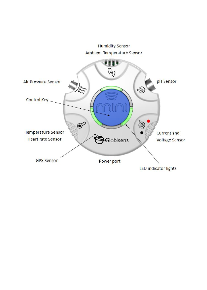
A left mouse click on the four bottom blue dot icons will
change the number of meters on the screen to: 1, 2, 4 or 6
meters. A left click on any of the meters will open a dialog
box for meter type selection and assigning a sensor for this
meter.
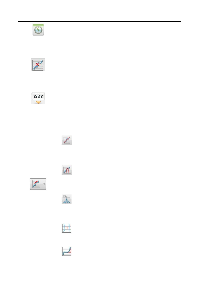
A left mouse click, near any of the graphs, will place a
marker on the graph. Hovering over any of the markers,
while pressing and holding the left mouse button and
dragging the mouse, will move the marker over the graph
and will show the values as the marker moves along the
graph line. Selecting the Marker icon again, exits the
Marker mode.
Allows a left mouse click to open a dialog box where text
and images can be entered. Pressing the Annotation icon
again exits the Annotation mode.
Pressing the Function-options small triangle icon allows the
user to apply the mathematical functions listed below
between the graph markers:
Linear regression will display the best linear line that
fits the graph between the locations of two markers. Next to
the line the software will open a small text box displaying
the linear line equation: Y= aX+b.
Quadric regression will display the best parabolic line
(2nd degree) that fits the graph between the locations of
two markers. Next to the line the software will open a small
text box displaying the parabolic line equation: Y= aX²+bX+c.
FFT is used to split the graphic display to show the
original measurements in a time scale in the top window
and to show its harmonics, on a frequency scale in the lower
window.
Smooth is used to average a graph. Every sample is
an average of the two readings before and two after
samples. It can be useful in case the graph is very noisy.
Derivative measures the sensitivity to change of a
quantity in one data source determined by another quantity
or another data source.