Optics11 Life PAVONE User manual

PAVONE
USER MANUAL

2optics11life.com
CONTACT INFORMATION
[phone]
[email protected]om
[email protected]om
www.optics11life.com
VISITING ADDRESS
VU University Campus
W&N Building room O-236
De Boelelaan 1081
1081 HV Amsterdam
The Netherlands
SHIPPING ADDRESS
De Boelelaan 1081
1081 HV Amsterdam
The Netherlands
COMPANY INFORMATION
Optics11 B.V.
KvK/CC: 52469417
VAT: NL850459734B01
Amsterdam, NL
Please see our website
for more information
about our products.
www.optics11life.com

3
CONTENTS
Revision history 4
Safety 5
Introduction 6
1. Installation 7
2. Preparing the setup for measurement 9
3. Using the Pavone 25
4. Additional system calibration and settings 48
5. Optimizing instrument stability and sample mounting 54
6. The OP1550 interferometer 58

4optics11life.com
REVISION HISTORY
Version 1.0 New document V1. March 4, 2019 Ernst Breel
Version 1.5 Update for V1.5.2 February 18, 2021 Nelda Antonovaite
Version 1.6 Update for V1.6.0 October 20, 2021 Ali Paknahad

5
SAFETY
The OP1550 interferometer, part of the Pavone instrument, is equipped with a class 1M laser. The laser
light is coupled out via a fiber connector on the front panel and has a terminator on the back panel. Do
not view directly into the beam with optical instruments.
The OP1550 is equipped with a 220V/110V plug. Disconnect the instrument before changing the fuse or
before switching from 220V to 110V (or vice versa). Do not open the box, as this might result in serious
injuries.
Water damage to the Pavone components is not covered by the warranty. Please make sure that no
liquids are spilled on the piezo, objective or other components.
PC of the Pavone is provided by the external supplier which includes operating system. Optics11 Life is
not responsible for the functioning of it. Please back up your data in case of malfunctioning of the PC or
operating system.

6optics11life.com
INTRODUCTION
This document describes the installation and operation of the Pavone instrument, as developed by
Optics11 Life (see Figure 1). Details of the installation of the Pavone are provided in Chapter 1. Chapter 2
describes the preparation of the Pavone and probes for experiments. How to perform the measurements
and operate the instrument is described in detail in Chapter 3. Chapter 4 describes how to calibrate
camera and microplates. Chapter 5 describes the optimization of sample preparation and measurement
conditions. Chapter 6 describes how to operate the OP1550 interferometer.
Figure 1: The Pavone in action: measuring microgels, organoids, cell cultures.

7
1. INSTALLATION
This section describes the general installation of the Pavone by providing an overview of its components,
the considerations for finding a location to set up the system, the wiring scheme for connecting the
individual components, and the actions required to start up the Pavone instrument. Please use a detailed
installation manual that was delivered with the system as there might be some system version-
dependent differences.
1.1 The Pavone and its components
The Pavone consists of (see Figure 2):
1. Pavone instrument body which also includes:
a. CCD Camera with the mount
b. Objective
2. Power supply unit
3. Interferometer OP1550
4. PC which also includes:
a. Keyboard and mouse
b. USB splitter
c. USB camera for remote training
5. Optics11 Life probes
Figure 2: Pavone main components.
For the best user experience, it is recommendedto first power on all separate components before running
the software.
1.2 Connecting components
Together with the Pavone instrument, the following cables are provided (some cables might be different
depending on the system configuration):
1. 2x power cables (for controller and interferometer)
2. 1x PC power cable including adapter
3. 3x USB 3.0 (A-B-type) cables
4. 1x USB 3.0 B –micro USB 3.0 B (camera type) cable
3
5
4
2
1
1.a

8optics11life.com
5. 1x BNC connector cable
6. 1x Pavone cable 26pin
7. 1x Intranet cable (maintenance)
8. 1x Patch cord cable (optical fiber)
Additional parts:
1. Piezo calibration probe and mirror
2. Screwdriver set
3. 24 empty wellplate
4. 6 wellplate Softwell
5. 50ml isopropanol and 3 pipettes
When installing the system, please carefully follow the scheme below (see Figure 3).
Figure 3: Schematic drawing of the connections that are required to set-up the Pavone instrument.
The power supply unit is connected to the Pavone using a special multi-pin power cable with a screw-on
type connector (see Figure 4). The Interferometer is connected using a BNC cable, to transmit the
outgoing optical signal to the acquisition electronics in the Pavone, and the USB-B cable to the PC,
allowing for communication with the Pavone through the PC. Pavone is connected to a PC with two USB-
B cables. The Camera, being a flexible component, connects to the PC through a separate micro USB cable.
Please note that all USB cables and connections should be of the USB 3.0 type: only connect to the PC’s
USB ports that have a blue-color USB port and use USB 3.0 certified cables. Failing to do so might cause
erratic system behavior. Connect patch cord fiber between OP1550 interferometer and Pavone which
shortens the cable length of the fiber of the probe for easier probe handling.
Figure 4: From left to right: patch cord and BNC cable connected to the interferometer, patch cord connection to Pavone,
mounted CCD camera and Pavone body connections.

9
2.PREPARING THE SETUP FOR MEASUREMENT
2.1 Starting the system
Powering up the instrument
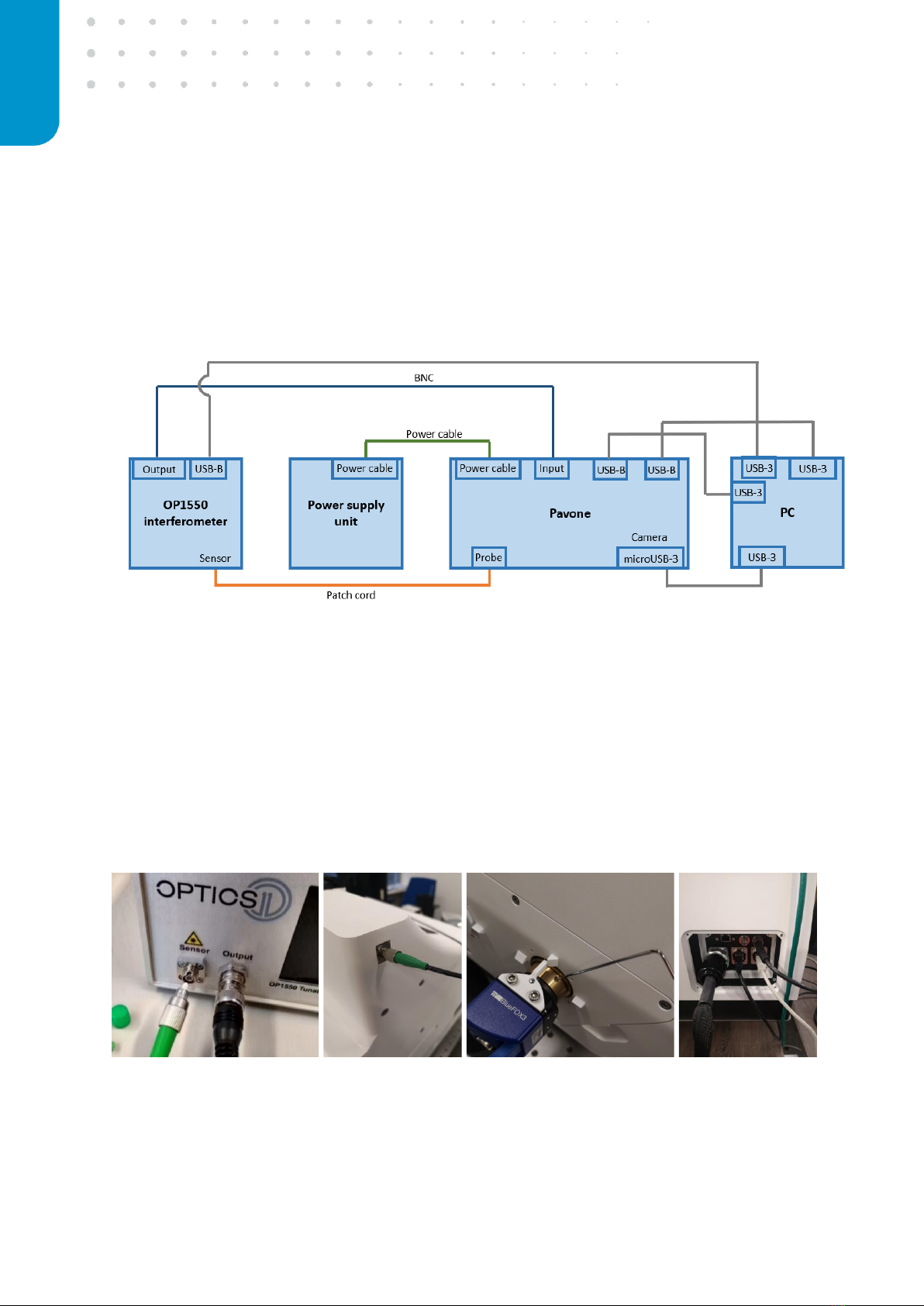
Before starting up the instrument for the first time, make sure that the stage lock is removed (follow the
installation manual provided with the system), all cables are connected correctly and the power switches
on the back of the boxes are turned on. Switch on the devices:
1. Interferometer
2. Power supply
3. PC
The interferometer will show a live measurement signal on the LCD screen after the initialization of the
laser is completed. The power supply unit automatically powers the Pavone unit.
Starting the software
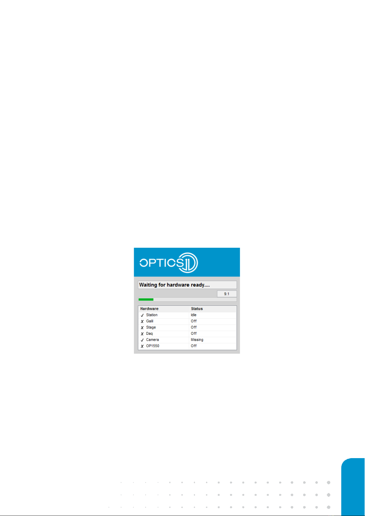
Ensure that stage locks are removed, nothing can obstruct sample stage movement. Start the Pavone
measurement software by double-clicking the Pavone software icon on the desktop. The software is
loading all devices while checking the hardware connection status, which should all be ‘Idle’ (see Figure
5) after a maximum waiting time of 60 seconds. The software will then proceed to the main user interface.
Figure 5: Hardware status check.
After starting the instrument the system will prompt homing of the XY sample stages: this is required to
‘zero’ the absolute position of the sample stages and ensure accurate positioning during use. After
homing the stages the system state will switch to ‘idle’.
2.2 Mounting a probe to the Pavone
Optics11 Life force sensors, also called probes, consist of optical fiber and cantilever (MEMS) that are
glued to glass ferrule perpendicularly. At the end of the cantilever, there is a spherical tip mounted either
directly on the cantilever or through an extended rod (see Figure 6). The spherical tip is used to deform

10 optics11life.com
the sample while optical fiber reads out cantilever bending during indentation. The cantilever acts as a
spring to measure the stiffness of the deformed material.
Figure 6: Force sensor (probe) design.
Selecting the right probe
Although a specific probe can measure a wide range of Young’s moduli, selecting a probe with suitable
parameters that match with the specific sample properties can enhance the quality of the measurement.
For a softer sample, a probe with a less stiff cantilever is needed, and vice-versa, to ensure that significant
cantilever bending as well as significant sample indentation is achieved during measurements. If the
probe is either too stiff or too soft, there will be minimal cantilever bending or indentation respectively,
resulting in a less optimal signal-to-noise ratio.
Advised cantilever stiffness is provided for ranges of sample Young’s moduli in the table below. These are
estimated for a tip radius of 25 µm, indentation depth of 2 µm. The full range is given considering
minimum cantilever bending of 0.01 µm and a maximum of 30 µm. The optimal range is given for
cantilever bending of 0.05 µm and a maximum of 20 µm.
Table 1: Young’s modulus and advised cantilever stiffness range (tip radius of 25 µm and indentation depth of 2 µm)
Full range of Young's modulus
Optimal range of Young's modulus
Advised cantilever stiffness range
10 Pa –30 kPa
50 Pa –20 kPa
0.025 N/m
100 Pa –298 kPa
500 Pa –199 kPa
0.25 N/m
2 kPa –6 MPa
10 kPa –4 MPa
5 N/m
20 kPa –59 MPa
99 kPa –39 MPa
50 N/m
60 kPa –179 MPa
298 kPa –119 MPa
150 N/m
For a tip radius of 3 µm and indentation-depth of 0.5 µm:
Table 2: Young’s modulus and advised cantilever stiffness range (tip radius of 3 µm and indentation depth of 0.5 µm)
Full range of Young's modulus
Optimal range of Young's modulus
Advised cantilever stiffness range
230 Pa –688 kPa
1.1 kPa –459 kPa
0.025 N/m
2.3 kPa –6.9 MPa
11 kPa –4.6 MPa
0.25 N/m
46 kPa –137 MPa
229 kPa –92 MPa
5 N/m

11
With a larger tip size, one can measure the lower stiffness range and vice versa. By indenting to larger
indentation depths, one can measure lower stiffness values. Use an excel sheet called “probe selection
calculator” to estimate the range of stiffness probe can measure for the given spring constant, tip size
and indentation-depth. In case of doubt, please do not hesitate to contact Optics11 Life for advice
([e-mail]). For the exact availability of probe stiffness and tip radius combinations,
check Optics11 Life webshop.
Installing a probe
Figure 7: Probe and fiber inside the probe box (left), probe mounting to the Pavone, fiber is connected to the adapter (right).
After powering the Pavone instrument, starting the software and homing the stages, a probe can be
mounted. To mount a probe, carefully open the probe box by ‘unclicking’ the four tabs holding the
transparent cover. Ensure any sticky tape is removed. Carefully take the probe out of the box in such a
way that the probe can be clicked in the probe holder in one go.
The probe is mounted in the Pavone instrument by compressing the probe’s spring by thumb and index
finger and gently pushing the probe with the holder in the probe mounting bay (see Figure 7). Make sure
the cantilever points downwards and the probe is mounted to the most back-right position. When
handling a probe, take special care to avoid any contact with the cantilever as the glass cantilever at the
end of the glass ferrule is extremely fragile and almost any unintended contact will cause permanent
damage. Therefore, when handling the probe, always hold it by the plastic adapter, keep the optical fiber
away from the cantilever and avoid touching the glass part. Given the size of the probe, it is advised to
hold the probe between ones’index finger and thumb. Hold your other fingers straight so that they are
away from the probe. Next, connect the fiber with the patch cord adapter. Make sure to hear the click
sound when connecting the fiber to the adapter.
Caution: Avoid bending the optical fiber sharply: this can break the glass fiber.
If a previous probe is present in the Pavone, remove it before inserting the new probe. To avoid the fiber
from touching the probe when packing the fiber and optical connector, always place the probe first and
then the fiber. Secure the optical connector in the box by placing a piece of tape on top of the connector.
You can remove the probe from the Pavone by compressing the plastic connector and pulling it gently
out of the holder. Carefully place the probe in the probe box to its designated location.
Caution: When installing the probe, always mount first the probe and then connect the
fiber connector to the Pavone connector. When putting the probe back into the box,
always place the probe first in and then the fiber.
Cantilever with tip

12 optics11life.com
2.3 Main software window and controls
Figure 8: Main Pavone components.
Y stage
X stage
100 µm piezo
probe stage
objective stage
plate 1
plate 2
probe
Cantilever
with tip
1
Piezo signal in V
Non-linearized cantilever signal in V
10
11
X stage
Y stage
2
3
4
5
6
8
7
9
Figure 9: Main software window.

13
Short description of main window controls (see Figure 8 and Figure 9):
1. Top window selection:
-Find Probe –allows calibration of probe tip position in respect to the camera image.
-Wellplates –allows moving to selected well in the plate.
-Calibration –calibration of the probe.
-Camera –camera settings and automatic image saving options.
-Options –settings for Find Surface and fitting of data.
-Config. exp. –set up indentation protocol and other steps.
-Maintenance –additional settings.
2. Probe stage controls:
-Single arrow –controls the step size of the probe stage and allows to move it up and down.
-Double arrow (Z up) –moves up the probe stage to 0 position.
-Incr. (µm) –step size.
-Set transit height –saves current probe stage position Z to “Transit(µm)”.
-Go to transit height –moves down the probe stage to the selected height in “Transit(µm)”.
3. Stage location:
-X(µm) –X stage coordinate.
-Y(µm) –Y stage coordinate.
-Z(µm) –probe stage coordinate.
-O(µm) –objective stage coordinate.
-“plate 1, A4” –current probe position within wellplate.
-Piezo (µm) –current position of the piezo together with the bar.
4. Microscopy:
-Bright field –turns on bright-field LED.
-Phase one –turns on phase-contrast LED suited for x20 objective.
-Phase two –turns on phase-contrast LED suited for x40 objective.
-LED intensity –adjusts LED intensity.
5. Temperature control:
-ON/OFF –turn on and off the temperature control.
-Set point (°C) –set temperature from 15 to 50°C.
-Air temp. (°C) –air temperature measured at the sensor (inside the frame).
-Humidity (%) –relative humidity.
6. Objective control:
-Auto cam adjust –automatically adjusts camera settings in “Camera” based on the current
image.
-Single arrow –controls thestep size of the objective stage and allows to move it up and down.
-Double arrow (objective down) –moves down the objective stage to 0 position.
-Incr. (µm) –step size.
-Set focal plane –saves current objective stage position Z to “Focal plane(µm)”.
-Go to focal plane –moves up the objective stage to the selected height in “Focal plane (µm)”.
7. Run experiment:
-Save image –saves the current camera image.
-Reset –resets all the hardware.
-Home stages –moves all stages to the initial position.

14 optics11life.com
-Stop –stops experiment or any other function.
-Run experiment –runs experiment set in “ Config. exp”
8. Move to point:
-Speed (µm/s) –approach speed that Z stage moves down during “Find Surface”.
-Z above surf. (µm) –the distance that the probe is retracted after the surface is found.
-Find Surface –moves Z-stage down until the surface is found.
-Threshold –defines the threshold value of cantilever deflection when the surface is detected.
9. Find surface:
-X(µm) –move to point X coordinate.
-Y(µm) –move to point Y coordinate.
-Move to point –executes the function.
-Speed (µm/s) –the speed at which XY stages move when running “Move to point” function.
-Coord.list –allows to set up a list of coordinates to be measured.
10. Live signals
-In blue –piezo position signal in Volts.
-In green –non-linearized cantilever position in Volts (the same as in interferometer
“Measure” window).
11. Camera feed and manual stage control:
-XY stage travel (µm) –step size when pressing arrows to move X and Y stages.
-Grabbing –frame rate of the camera
-Scale bar

15
2.4 Calibration sequence
When starting to work with the Pavone, three steps are required to calibrate the system:
In the software these three steps are indicated in the top menu:
Each button opens a menu enabling specific actions. In general, the sequence to follow is from left to
right. In the paragraphs below each step is explained in more detail.
2.5 Find probe: in air
To couple indentation location with imaging data, the reference point of the probe tip is used. Follow the
steps:
1. To start the procedure, mount the probe, leave plate 1 empty.
2. Move Y-stage by 30 000 µm so that objective is easily accessible and can move up without
obstructions.
3. Move probe stage Z down by ~20 000 µm. Move objective stage O up in steps of 500 or 1000 µm.
4. Rotate a metal screw above the probe stage to loosen up manual XY stage knobs (seeFigure 10,
left image). Using the knobs (see Figure 10, second image from the left), align the probe first by
eye until the cantilever tip is hovering above the center section of the objective (see Figure 10,
images on the right).
5. Turn on “Brightfield”and “Phase 2”and press “Auto cam adjust”in the software. If the image of
the camera is dark, increase LED intensity or go to “Camera” settings. You should see an image or
shadow of the probe. If necessary, adjust the height of the objective stage so that the probe is in
the focal plane (check the working distance of your objective e.g. Nikon WD 3.1 mm for x20
objective, WD 2.1 mm for x40 objective).
6. Continue alignment of the probe with manual knobs until you see the end of the cantilever as in
Figure 11. Use small steps of the objective stage to get the tip of the probe in focus. Position the
tip at the top of the field of view of the camera.
7. Tighten back the top screw.
8. Press “Find Probe”in software, use the circle tool to mark the circumference of the tip (see Figure
11). Tip: press and hold SHIFT while doing so to keep a perfect circle during resizing. After
Find probe Wellplates Calibration
Find probe Wellplates Calibration
Click in
probe
Move Y
stage
down
Move Z-
stage
down
Move O-
stage up
Adjust
manually
probe
Focus on
the tip Find Probe

16 optics11life.com
confirming the tip location, press save. Keep in mind that tip position in the camera view will
deviate depending on the Z-stage position (>10µm along 2000 µm change in Z-stage)
9. Before commencing with the next steps, click ‘Home stages’ in the ‘Controls’ tab once, to move
all stages to a safe position for sample plate mounting.
Caution: When using high magnification objectives please ensure that the objective is
not touching the probe.
Caution: Please ensure to untighten the black knob at the top of the condenser before
adjusting the probe position and tighten again after adjustment.
Figure 10: From left to right: knob to release manual stages circled in red; manual micromanipulators for probe adjustment
circled in red: top one moves horizontally (along X axis) and bottom one moves vertically (along Y axis); checking probe position
by eye along X and Y axis.

17
Figure 11: Locate tip menu. The red circle marks the tip position (top 25 µm radius tip and bottom 3 µm radius tip). You can use
the zoom function for smaller tips.
2.6 Configuring sample plates
After the probe is aligned, the sample plates can be mounted and configured in the software. The
software allows loading different well plate formats (for more information see Section 4.1). With the
delivery of the system, an empty “costar 24 well plate” is provided which dimensions are already
calibrated. Please use it until you get more familiar with the system. Other calibrated well plates are:
-96 and 24 microplates from Greiner (LINK).
-96 and 6 Softwell plates from Matrigen (LINK).
Follow these steps:
1. First, mount the microplate by pushing it down until all sides touch the bottom of the plate holder
and the plate feels firm in the X direction (there are springs on the right side that keep the plate
firm). If the microplate can move in the Y direction, push it to the top. Choose the well that will
act as the calibration well, it should be loaded without any sample, only filled with the same liquid
as used for the samples such as phosphate-buffer saline (PBS), water, culture medium, or just air,
and has a clean and hard surface at the bottom, without any coating which would make it sticky.
Find probe Wellplates Calibration
Mount sample
plate(s) Wellplates Select calibration well Move to calibration well

18 optics11life.com
Caution: The probe is sensitive to the refractive index of the medium and
temperature, thus, the probe needs to be calibrated in the same medium as the
sample and at a stable temperature.
2. Open the “Wellplates” menu which will show the two sample docks (see Figure 12). To configure
your sample plates, select the right sample plate format from the drop-down menu. Select the
calibration well by pressing on the well (e.g. A1).
3. Press “Move to well” and the stage will adjust the position so that the probe is above the selected
well. Then, move down the probe by pressing the probe stage down at steps of 1000 µm and
check that the probe is going to enter the well at the top left corner without hitting the edge of
the well (see Figure 13, left image). If the probe position with respect to the well is not correct,
calibrate the wellplate (see Section 4.1).
4. Prewet the probe by pipetting the medium (the same solution as used in the calibration well)
over the front face of the probe until you can clearly observe a droplet hanging underneath the
probe, see Figure 13, right image. This will minimize the risk of trapping air bubbles underneath
the cantilever. During prewetting droplets of medium or water may fall in the underlying well.
Caution: It is recommended to clean the probe with isopropanol followed by water
before calibration to remove electrostatic charges, residue and decrease surface
tension.
Figure 12: “Config. wells”menu which allows bringing the probe above the selected well. Wells need to be calibrated for their
dimensions (see Section 4.1).

19
Figure 13: Probe is entering at the top left corner of the well (left image), and probe is being preweted by pipetting liquid down
the probe front-face (right image).
2.7 Initialize probe
Before the use of the probe, the laser inside the interferometer and geometrical factor of the probe must
be calibrated as it is unique for each probe and medium. This process must be performed for each new
medium/probe combination: to measure multiple samples in a solution of which the refractive index is
not significantly different, this procedure does not have to be executed again. Follow these steps:
1. Input the probe parameters in the software suite to obtain meaningful measurement results.
Probe parameters that need to be set in the program are the cantilever spring constant k (N/m)
and probe tip radius R (µm). These parameters can be entered in the ‘Calibration’meniu, see
Figure 14. The numbers can be found on the side of the probe packaging box and are unique for
each probe. They are calibrated in the air by indenting on a scale
1
. If you accidentally forget to
update the probe details after changing the probe, you can still change those in the DataViewer
software while analyzing the obtained data.
1
Beekmans, S. V., & Iannuzzi, D. (2015). A metrological approach for the calibration of force transducers with interferometric
readout. Surface Topography: Metrology and Properties, 3(2), 025004. https://doi.org/10.1088/2051-672X/3/2/025004
Find probe Wellplates Calibration
Probe details Wavelength
scan Find surface Calibrate

20 optics11life.com
Figure 14: Probe calibration menu.
2. Move the probe to the calibration well using ‘Wellplates’window.
3. Make sure that the probe is prewetted.
4. Now you should move down the probe in “Incr. (µm)” steps of 5000 µm until the probe is clearly
below the liquid level “Z(µm)”~15 000 µm. If needed, fill the well with more medium so that the
probe is clearly submerged but not too close to the bottom of the well or too close to the surface
of the liquid.
5. Wait a few minutes so that the probe can adjust to the new environment. When performing
experiments with temperature control, the calibration should be accomplished at the same
temperature as the measurement temperature. This is because probe is sensitive to temperature
variations.
6. Click the “Scan OP1550 Wavelength”button once. The interferometer screen will now show a
progress bar. The live signal window on the screen show oscillations, see Figure 15-b (zoom in if
needed). Wait until that is finished and check if no error (see Figure 15-d) is reported on the
interferometer screen or software. You can also check the final result of the “Wavelength scan”
in the corresponding interferometer window 15-c.