Quanser 6 DOF Hexapod User manual

6 DOF Hexapod
Laboratory Guide
Hexapod
Quanser Inc.
2016

c
2016 Quanser Inc., All rights reserved.
Quanser Inc.
119 Spy Court
Markham, Ontario
L3R 5H6
Canada
[e-mail]
Phone: [phone]
Fax: [phone]
Printed in Markham, Ontario.
For more information on the solutions Quanser Inc. offers, please visit the web site at:
http://www.quanser.com
This document and the software described in it are provided subject to a license agreement. Neither the software nor this document may be
used or copied except as specified under the terms of that license agreement. All rights are reserved and no part may be reproduced, stored in
a retrieval system or transmitted in any form or by any means, electronic, mechanical, photocopying, recording, or otherwise, without the prior
written permission of Quanser Inc.
HEXAPOD Laboratory Guide 2

Contents
1 Introduction 4
2 Running the 6 DOF Hexapod 5
2.1 Calibration 5
2.2 Homing 6
2.3 Joint-Level Position Control 7
2.4 World-Space Position Control 9
2.5 Brake Bypass 12
2.6 Earthquake 13
2.7 FFT Analysis 15
2.8 Hexapod Controllers 16
3 Background 23
3.1 Modeling 23
3.2 Position Controller Design 23
3.3 Downloading New Earthquakes 24
4 System Requirements 26
4.1 Overview of Files 27
4.2 Setup script: setup_hexapod.m 28
4.3 Creating an Earthquake: make_quake_xyz.m 30
HEXAPOD Laboratory Guide v 1.3

1 INTRODUCTION
This laboratory manual describes how to use the Quanser 6 DOF Hexapod QUARC controllers. See the 6 DOF
Hexapod User Manual [2] for information about the hardware setup (i.e., connections) and specifications.
Topics Covered
•Calibrating the Hexapod on power up.
•Moving the upper stage or platform to the HOME position (i.e., where linear actuator are in center or mid-stroke
position).
•Running joint-level and world-space position controls on the 6 DOF Hexapod.
•Transfer function model of the linear actuator.
•PID-based controller used to control position of stage.
Prerequisites
In order to successfully carry out this laboratory, the user should be familiar with the following:
1. See the system requirements in Section 4 for the required hardware and software.
2. Modeling and transfer function representation.
3. PID control design.
4. Basics of Simulinkr.
5. Basics of QUARCr, i.e., how to build/run a Simulink model in QUARC.
HEXAPOD Laboratory Guide 4

2 RUNNING THE 6 DOF HEXAPOD
This section explains how to use the supplied Simulinkrmodels with the QUARCrsoftware to run the following
controllers on the Hexapod:
1. Calibration - Runs an auto routine on all the drives and resets the encoders to zero. Required after system
power up.
2. Home - Positions the Hexapod to the HOME position where each joint is at the mid-stroke position. Make sure
the Hexapod is at home BEFORE running the regular controller (e.g., joint position control).
3. Joint Level Control - Control the position of the base joints at the linear actuator level.
4. World Space Control - Control the X, Y, Z, Roll, Pitch, and Yaw position of the top stage.
5. Brake Bypass - Releases the brake system to move the stage manually.
6. Earthquake - Run scaled down version of a recorded earthquake on the table, e.g., Northridge or Kobe earth-
quake.
Note: All the supplied controllers are already configured for the hexapod2_usb data acquisition (DAQ)
device. If you are using these files on different DAQ or system, then see the QUARC User Manual [1] for instructions
on how to change Board type in the HIL Initialize block.
2.1 CALIBRATION
When the Hexapod is first powered ON, the positions measured from the encoders on all the joints are reset to 0,
regardless of where the base joint of the Hexapod are actually at. The Hexapod_Calibrate.mdl controller, shown
in Figure 2.1, positions each of the six joints along the linear guide until they reach the limit switch. Once all six
joints have been placed at the limit switch positions, the encoders are reset and the model is stopped. If the joints
are already at the calibrated position then the controller will only reset the encoders and stop the controller. Once
calibrated, run the homing procedure outlined in Section 2.2.
Caution: Calibration must be performed EVERY TIME the Hexapod is powered ON and before ANY other
controller!
HEXAPOD Laboratory Guide v 1.3

Figure 2.1: Simulink model used to calibrate the 6 DOF Hexapod using QUARC.
Follow these steps to calibrate the system:
1. Make sure the red button is in the upper position to enable the amplier. The amplier cannot be enabled when
the button is in the lower position. Twist the button to ensure it is in the enabled position.
2. Open the Simulink model called Hexapod_Calibrate.mdl, shown in Figure 2.1.
3. Run setup_hexapod.m in MATLAB (note: script is ran automatically when Simulink model is ran).
4. Click on QUARC | Build to generate the controller.
5. Power ON the Hexapod system by placing the power switch to the ON position.
6. Run the QUARC controller by going to QUARC | Start. Each of the base joints should move to their limits until
the limit switches are triggered.
Caution: PRESS DOWN on the RED BUTTON of the E-Stop switch to stop the Hexapod. This
deactivates the amplifier and cuts off the DC motor power.
7. The controller stops automatically when each of the six joints have reached their limit switch.
2.2 HOMING
Before running Hexapod_Joint_Control.mdl, Hexapod_World_Control.mdl, or any other position-based experiments,
the stage of the 6 DOF Hexapod must be in the HOME position. This is defined when each base joint is at its mid-
stroke position. The Hexapod_Home.mdlSimulink model, shown in Figure 2.2, is ran with QUARC to center all the
linear joints at the base.
HEXAPOD Laboratory Guide 6

Figure 2.2: Simulink model used to home the Hexapod using QUARC.
Follow these steps to home the system:
1. Make sure the red button is in the upper position to enable the amplier. The amplier cannot be enabled when
the button is in the lower position. Twist the button to ensure it is in the enabled position.
2. Make sure you have calibrated the Hexapod first, as described in Section 2.1.
3. Open the Simulink model called Hexapod_Home.mdl, shown in Figure 2.2.
4. Run setup_hexapod.m in MATLAB (note: script is ran automatically when Simulink model is ran).
5. Click on QUARC | Build to generate the controller.
6. Run the QUARC controller by going to QUARC | Start. The upper stage should move to the HOME position
when are all the linear actuator are in the mid-stroke or center position.
Caution: PRESS DOWN on the RED BUTTON of the E-Stop switch to stop the Hexapod. This
deactivates the amplifier and cuts off the DC motor power.
7. The controller stops automatically when the HOME position is reached.
2.3 JOINT-LEVEL POSITION CONTROL
This Hexapod_Joint_Control.mdlcontroller shown in Figure 2.3 applies position commands to the base-level linear
actuators. The user can specify the amplitude and frequency of the sine wave on-the-fly and read corresponding
position measurements.
HEXAPOD Laboratory Guide v 1.3

Figure 2.3: Simulink model used to command joint-level positions to the 6 DOF Hexapod using QUARC.
The joint commands can be found inside the Desired Joint Reference \Desired Joint Reference subsystem block
shown in Figure 2.4. The home reference of 176.5 mm is applied to each joint .
The home reference command are set in the Slider Gain blocks shown in Figure 2.4a. The Periodic Wave Commands
subsystem, shown in Figure 2.4b, has Slider Gain blocks that are, by default, all initially set to zero. Change their
values in order to apply a sine wave command.
(a) HOME reference command (b) Sine or square wave position commands
Figure 2.4: Hexapod position commands
Caution: Make sure the Hexapod is at the HOME position before running this experiment! If the joints
are not at the mid-stroke or center position, then go through the homing procedure in Section 2.2.
Follow these steps to run the controller:
1. Make sure the Hexapod is at the HOME position, as described in Section 2.2.
2. Make sure the red button is in the upper position to enable the amplier. The amplier cannot be enabled when
the button is in the lower position. Twist the button to ensure it is in the enabled position.
HEXAPOD Laboratory Guide 8

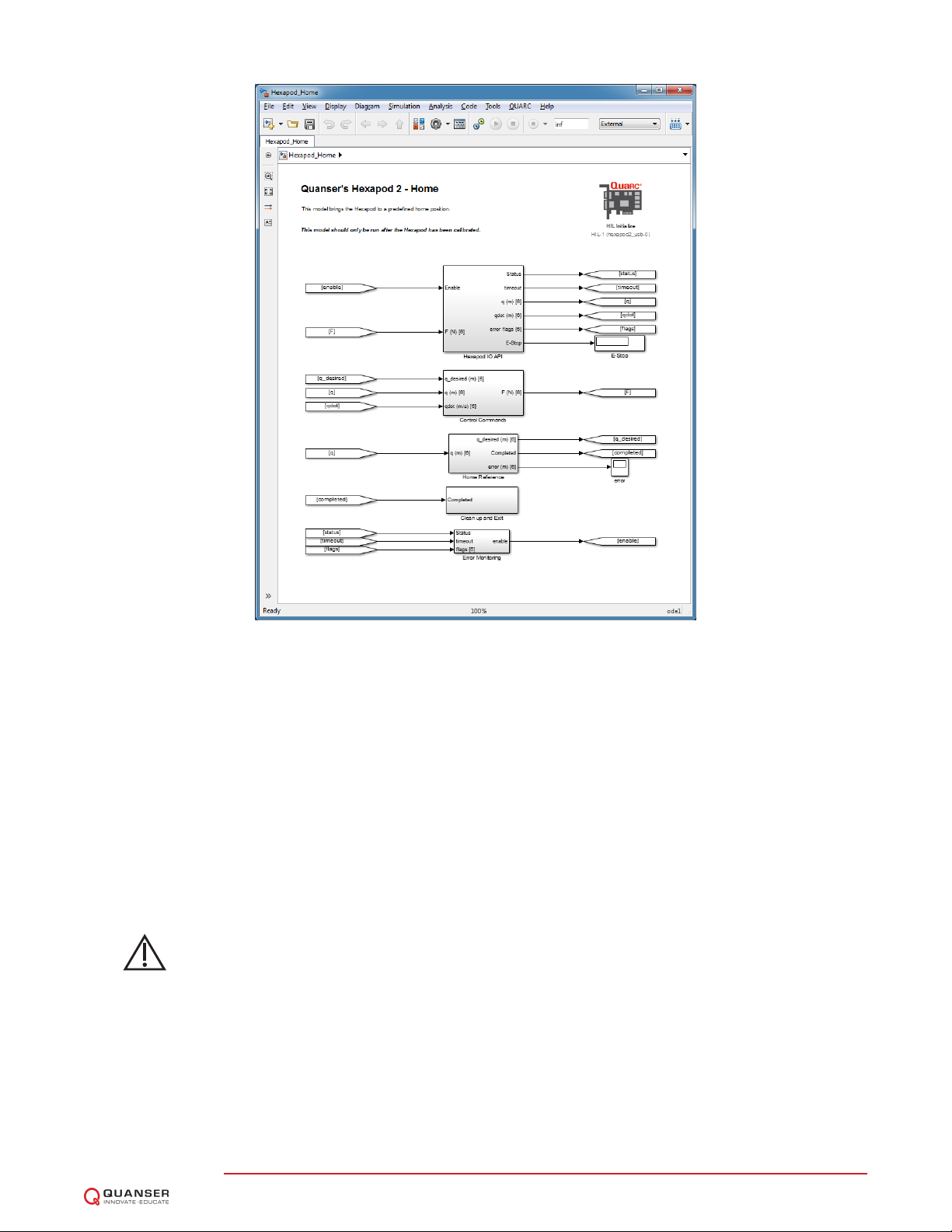
3. Open the Simulink model called Hexapod_Joint_Control.mdl, shown in Figure 2.3.
4. Run setup_hexapod.m in MATLAB (note: script is ran automatically when Simulink model is ran).
5. Click on QUARC | Build to generate the controller.
6. Run the QUARC controller by going to QUARC | Start.
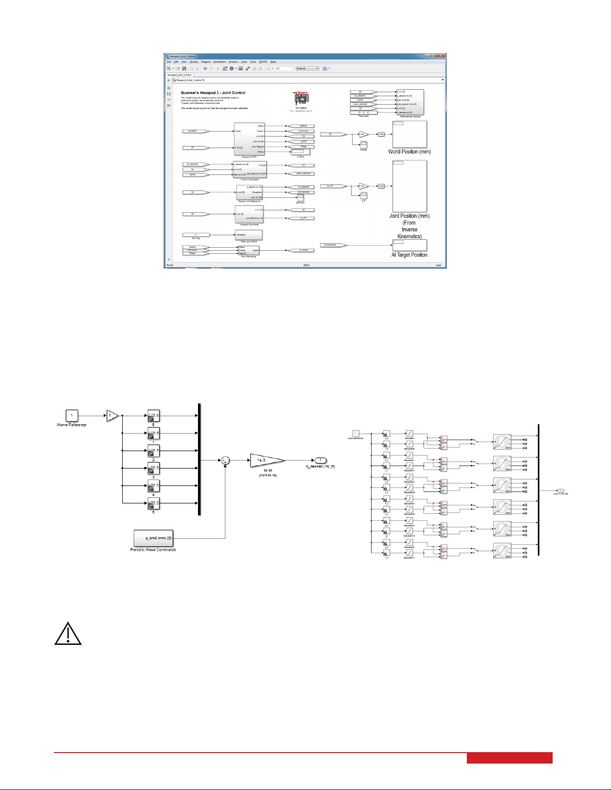
7. Change the values of the Slider Gain blocks in in the Figure 2.4b gradually to begin commanding a sine wave
to the linear actuators.
Caution: PRESS DOWN on the RED BUTTON of the E-Stop switch to stop the Hexapod. This
deactivates the amplifier and cuts off the DC motor power.
8. Open the Joint Position Tracking and Joint Speed Tracking scopes, located in the Performance Tracking sub-
system, to examine the position or speed response of the Hexapod. The yellow trace is the measured posi-
tion/speed and the purple plot is the desired position/speed. To change which joint position/speed is being
displayed, set the Joint Index block between 1 and 6 accordingly. See Section 2.8.5 for more information.
9. Before stopping the controller, it is recommended to set position commands back to the home reference. That
is, set the Slider Gain blocks in the Periodic Wave Commands subsystem in Figure 2.4b all to 0 and the Constant
block in Figure 2.4a to 140 mm to bring the stage back to HOME position and ready for the next experimental
run.
Note: The Constant and Slider Gain block values for the setpoint commands are automatically reset to the
home reference automatically when the controller is stopped. However, because this is performed after the
controller is stopped, it does not physically move the platform back to HOME. This must be done manually as
the controller is still running.
10. Click on Stop button in the Simulink diagram tool bar to stop running the controller.
11. Shut off the Hexapod power switch if no more experiments will be conducted.
Note: As explained in the Hexapod User Manual [2], if a limit switch is triggered the amplifier automatically stops
accepting any motor/joint commands in that direction. However, position commands in the opposite direction are still
accepted (e.g., joint can be moved back to home).
The forward and inverse kinematics are included in Hexapod_Joint_Control.mdl to provide a comparison between
the measured joint positions, and those obtained using the derived kinematics. The World Position display block can
be used to monitor this world coordinate position. The Inverse Kinematics block is used to find the six joint positions
given the measured world coordinate position of the end-effector (i.e., the output from the Forward Kinematics block).
This joint space position vector can be monitored in the Hexapod Joints (From Inverse Kin) display and compared
to the actual joint positions shown in the Hexapod Joints display. See Section 2.8.4 for more information about the
kinematic blocks.
2.4 WORLD-SPACE POSITION CONTROL
This Hexapod_World_Control.mdl controller shown in Figure 2.5 controls the position of the upper stage, i.e., the
end-effector. The amplitude and frequency of the sine or square wave can be adjusted for each of the end-effector’s
axes: X, Y, Z, Pitch, Roll, and Yaw.
HEXAPOD Laboratory Guide v 1.3

Figure 2.5: Simulink model used to command world-space positions to the 6 DOF Hexapod using QUARC.
The end-effector world coordinate commands are given in the Desired Position Reference subsystem block shown
in Figure 2.6. The setpoint for each of the end-effector’s axes - X, Y, Z, Pitch, Roll, and Yaw - can be set to either a
sine wave or square wave. Set the amplitude and frequency of the signal using the Slider Gain blocks. For example,
set gain block A_x to 2 and gain block f_x to 0.5 to apply a ±2 mm sine wave at 0.5 Hz.
HEXAPOD Laboratory Guide 10

Figure 2.6: Hexapod world coordinate position commands
Caution: Make sure the Hexapod is at the HOME position before running this experiment! If the joints
are not at the mid-stroke or center position, then go through the homing procedure in Section 2.2.
Follow these steps to run the controller:
1. Make sure you have home the Hexapod first, as described in Section 2.2.
2. Make sure the red button is in the upper position to enable the amplier. The amplier cannot be enabled when
the button is in the lower position. Twist the button to ensure it is in the enabled position.
3. Open the Simulink model called Hexapod_World_Control.mdl, shown in Figure 2.5.
4. Run setup_hexapod.m in MATLAB (note: script is ran automatically when Simulink model is ran).
5. Click on QUARC | Build to generate the controller.
6. Run the QUARC controller by going to QUARC | Start.
7. Change the values of the Slider Gain blocks in the Desired Position Reference block, shown in Figure 2.6
subsystem, gradually to begin commanding a position command to the top stage.
Caution: PRESS DOWN on the RED BUTTON of the E-Stop switch to stop the Hexapod. This
deactivates the amplifier and cuts off the DC motor power.
8. Open the World Position Tracking scopes in the Performance Tracking subsystem to examine the position
response of the Hexapod end-effector. The yellow trace is the measured world coordinate position and the
purple plot is the desired position. To change which axes is being displayed, set the Position Index block
between 1 and 6 accordingly. See Section 2.8.5 for more information.
9. Before stopping the controller, it is recommended to set the sine/square wave amplitudes back to 0 to HOME
the Hexapod so it is ready for the next experimental run.
HEXAPOD Laboratory Guide v 1.3

Note: The Slider Gain values are actually reset to the home reference automatically when the controller is
stopped. The signal amplitude gains are all reset to 0 and the frequency gain blocks are set back to 1 Hz.
However, because this is performed after the controller is stopped, it does not physically move the platform
back to HOME. This must be done manually as the controller is still running.
10. Click on Stop button in the Simulink diagram tool bar to stop running the controller.
11. Shut off the Hexapod power switch if no more experiments will be conducted.
Note: As explained in the Hexapod User Manual [2], if a limit switch is triggered the amplifier automatically stops
accepting any motor/joint commands in that direction. However, position commands in the opposite direction are still
accepted (e.g., joint can be moved back to home).
The measured end-effector position, from the Forward Kinematics block is shown in the World Position (mm) display
block. The measured joint positions are shown in the Joint Position display.
2.5 BRAKE BYPASS
The Hexapod_Brake_Bypass.mdl model, shown in Figure 2.7 allows the joints to be moved manually. The amplifier
drives are enabled and the brake system is disabled when the Digital Output Channels #12 and #13 are set to 0
and 1, respectively. The amplifiers are disabled when the DO #12 and #13 are both set to 1. The joints can be
moved manually as long as the amplifiers are enabled (and no internal amplifier faults, such as over-current or
over-temperature are triggered).
Figure 2.7: Simulink model used to disengage brakes on the Hexapod using QUARC
Follow these steps to disengage the brake system:
1. Make sure the red button is in the upper position to enable the amplier. The amplier cannot be enabled when
the button is in the lower position. Twist the button to ensure it is in the enabled position.
2. Open the Simulink model called Hexapod_Brake_Bypass.mdl, shown in Figure 2.7.
3. Run setup_hexapod.m in MATLAB (note: script is ran automatically when Simulink model is ran)..
HEXAPOD Laboratory Guide 12

4. Click on QUARC | Build to generate the controller.
5. Power ON the Hexapod system by placing the power switch to the ON position.
6. Run the QUARC controller by going to QUARC | Start. The base joints should now be free to move manually.
Caution: PRESS DOWN on the RED BUTTON of the E-Stop switch to stop the Hexapod. This
deactivates the amplifier and cuts off the DC motor power.
7. Click on Stop button in the Simulink diagram tool bar to stop running the controller. This engages the deactivates
the amplifier and engages the brake system.
8. Shut off the Hexapod power switch if no more experiments will be conducted.
2.6 EARTHQUAKE
The Hexapod_Earthquake.mdl Simulink diagram shown in Figure 2.8 can be used to replay earthquake on the 6
DOF Hexapod system using QUARCr. Recorded earthquake data, i.e., data collected when an actual earthquake
occurred, can be scaled down and ran on the Hexapod. Four historical earthquakes have been supplied for the user:
Northridge, Kobe, El-Centro, and Mendocino. For instructions on how to download new earthquakes, see Section
3.3. The user can also specify and create a pre-defined compound sine wave trajectory.
Figure 2.8: Simulink model used to command earthquake to the 6 DOF Hexapod using QUARC.
Caution: Make sure the Hexapod is at the HOME position before running this experiment! If the joints
are not at the mid-stroke or center position, then go through the homing procedure in Section 2.2.
1. Make sure the red button is in the upper position to enable the amplier. The amplier cannot be enabled when
the button is in the lower position. Twist the button to ensure it is in the enabled position.
2. Open the Simulink model called Hexapod_Earthquake.mdl, shown in Figure 2.8.
3. Run setup_hexapod.m in MATLAB. Note: script is NOT ran automatically like other models - this must be ran
manually.
HEXAPOD Laboratory Guide v 1.3

4. The command position (and acceleration) must first be loaded into the MATLAB environment. Select your
earthquake record and run the make_quake_xyz.m script to load the scaled data. For more information
about using the make_quake_xyz.m script, see Section 4.3.
5. Click on QUARC | Build in Hexapod_Earthquake.mdl to generate the controller.
6. Run the QUARC controller by going to QUARC | Start. The top stage should begin tracking the loaded earth-
quake (or sine wave).
Caution: PRESS DOWN on the RED BUTTON of the E-Stop switch to stop the Hexapod. This
deactivates the amplifier and cuts off the DC motor power.
7. Typical position and acceleration responses when running the Northridge earthquake is shown in Figure 2.9
for the x-axis.
(a) Position along X-Axis
(b) Measured Acceleration along X-Axis (c) Computed Acceleration along X-Axis
Figure 2.9: Hexapod stage position and acceleration when running Northridge earthquake.
8. The controller stops by itself when the duration of the earthquake (or sine) is reached. The controller can be
stopped, however, by clicking on the Stop button in the Simulink diagram tool bar at any time.
9. Shut off the Hexapod power switch if no more experiments will be conducted.
10. To plot the FFT of the position or acceleration, run fft_eval_pos.m or fft_eval_acc.m. See Section 2.7 for
instructions.
HEXAPOD Laboratory Guide 14

Note: As explained in the Hexapod User Manual [2], if a limit switch is triggered the amplifier automatically stops
accepting any motor/joint commands in that direction. However, position commands in the opposite direction are still
accepted (e.g., joint can be moved back to home).
2.7 FFT ANALYSIS
This section shows how to evaluate the power spectrum of the commanded and measured Hexapod position and
acceleration signals using the fft_eval_pos.m and fft_eval_acc.m scripts. Given a time-based signal g(t), the power
spectrum shown on the plot generated is given by |G(ω)|, where G(ω)is the Fast-Fourier Transform (FFT). The FFT,
G(ω), is computed using the Matlabr t command. See the power_spectrum.m script for further details.
1. Run an earthquake or sine wave using the Hexapod_Earthquake.mdl QUARC controller, as described in Sec-
tion 2.6. After Hexapod_Earthquake.mdl is ran, the commanded and measured position and acceleration data
are automatically saved to the Matlab data files data_xyz_pos.mat and data_xyz_acc.mat. Only one axis is
saved to these variables - either X, Y, or Z - depending on the selection in the Position Index block found in the
Performance Tracking subsystem, as shown in Section 2.8.5.
2. To produce the |X(ω)|position power spectrum similar to Figure 2.10, run fft_eval_pos.m. The desired or
commanded position is the blue trace and the measured position (from the encoder) is the red plot line.
Figure 2.10: FFT of desired and measured position along x-axis after running Northridge earthquake
3. To produce the acceleration power spectrum, A(ω), similar to Figure 2.11, run fft_eval_acc.m. The blue and
red traces are the desired and measured accelerations, respectively.
HEXAPOD Laboratory Guide v 1.3

Figure 2.11: FFT of desired and measured acceleration along x-axis after running Northridge earthquake
4. In both the fft_eval_pos.m and fft_eval_acc.m scripts, you can adjust the frequency range by adjusting the
f_min and f_max variables:
% min/max frequencies for plotting (Hz)
f_min = 1;
f_max = 10;
2.8 HEXAPOD CONTROLLERS
This section briefly describes some of the blocks used the Simulink models that are supplied with Hexapod, to be
used with QUARC. Some of the blocks designed specifically for the Hexapod are found in the Hexapod_Library
Simulink library, depicted in Figure 2.12.
HEXAPOD Laboratory Guide 16

Figure 2.12: Hexapod library used in QUARC controllers supplied
2.8.1 Position Reference
As shown in Figure 2.13, the Hexapod positions commands are smoothed in the Home Reference \Trajectory
Smoothing subsystem. The Linear Trajectory block takes in the desired position of each joint, the initial joint po-
sitions as well as the maximum allowed speed for each joint. The block then outputs a calculated trajectory for each
joint to follow. This trajectory is the position command to each joint.
Figure 2.13: Hexapod position commands are smoothed and checked for collisions
The position references go through the collision avoidance logic to prevent adjacent joints from colliding with each.
HEXAPOD Laboratory Guide v 1.3

This is done by keeping a minimum distance between them. The separation distance can be set in setup_hexapod.m
in the min_separation variable. Note that this is defined as the distance between the joint center to joint center - not
the side to side distance. Furthermore, each joint is limited to maximum and minimum position using a Simulink Sat-
uration block. Additional checks are included to detect and avoid potential collisions caused by the desired position
references between the links and the mounting brackets at each joint location. The desired position references will
be passed through the Joint Collision Avoidance subsystem if they do not result in a collision condition. Otherwise,
the previous desired joint commands will be held until a set of collision-free desired position references are received
(and be passed through).
2.8.2 Hardware Interface
The QUARC blocks used to interface to the Hexapod amplifier, linear actuators, and encoders is done, at a higher-
level, in the Hexapod IO API subsystem shown in Figure 2.14.
HEXAPOD Laboratory Guide 18

Figure 2.14: Hexapod IO API subsystem
The Hexapod HW API subsystem, depicted in Figure 2.15, includes the hardware blocks that interface directly to
the hardware actuator and sensors. The HIL Read Timebase block reads the six encoders, status of all six amplifier
drives (e.g., if a fault occurs), and the encoder velocities. Using the Timebase block forces the controller to use the
clock from the data acquisition device for more deterministic sampling when running the controller (as opposed to the
PC system timer). The HIL Write enables the amplifiers and applies the PWM amplitude and direction commands
to the amplifier drives. Finally, HIL Watchdog monitors the controller performance and stops it if a timeout occurs.
HEXAPOD Laboratory Guide v 1.3

Figure 2.15: QUARC blocks used to interface to Hexapod actuators and sensors
The Hexapod IO API \Hexapod IO subsystem, shown in Figure 2.16, interfaces Hexapod position controller to the
the hardware I/O explained above. For instance, it converts the encoder counts to joint linear position (i.e., multiplied
by the encoder resolution and motor shaft circumference constant). Based on the force computed by the Hexapod
controller to reach the desired position, denoted as F, this subsystem computes the current required for the amplifier
drives (see Section 3.2 for the force to current conversion).
The current is converted to the PWM signals required. The PWM magnitude is applied to the QUARC HIL Write
block on PWM Channels #0 to #5 and the PWM direction is applied to DO Channel #0 to #5. Note that current
commands are saturated according the configured amplifier limits to help prevent the motors or amplifier drives from
over-heating (see Hexapod User Manual [2] for current limit specifications).
Figure 2.16: Hexapod IO subsystem
HEXAPOD Laboratory Guide 20