6/18 Bosch Rexroth AG Hydraulics HAB RE 50170/01.09
0,1
0,6
0,7
0,8
0,9
1,0
0,2 0,3 0,4 0,5 0,6 0,7 0,8 0,9 1,0
p
2
= 300 bar
p
2
= 200 bar
0,1
0,6
0,7
0,8
0,9
1,0
0,2 0,3 0,4 0,5 0,6 0,7 0,8 0,9 1,0
P1/ P2
Ki
Application of the calculation diagrams
(see pages 7 to 10)
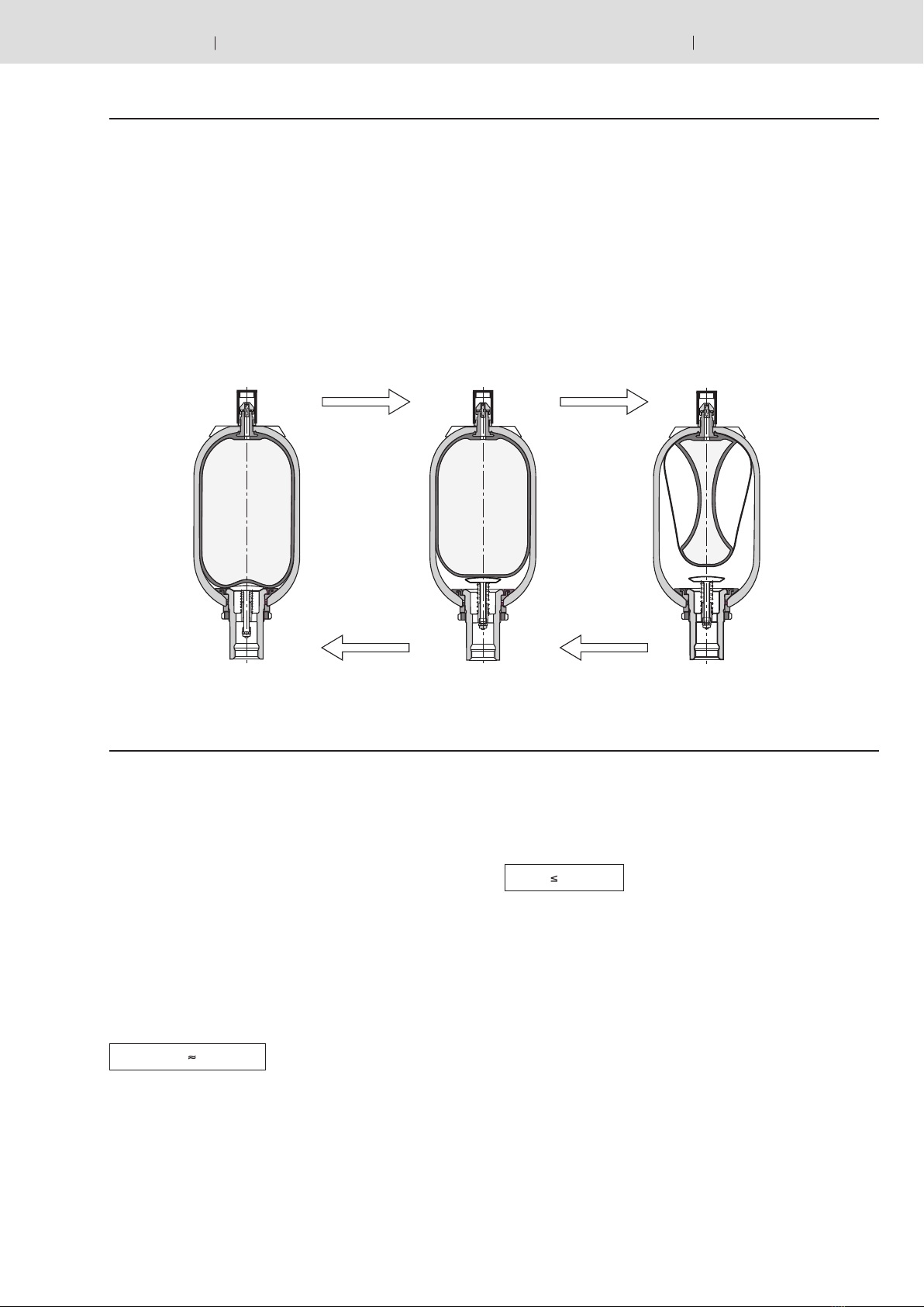
Calculation
Oil volume
Pressures p0… p2determine gas volumes V0… V2.
Here, V0 is also the nominal capacity of the accumulator.
The available oil volume Vcorresponds to the difference be-
tween gas volumes V1and V2:
The gas volume, which is variable within a pressure differential,
is determined by the following equations:
a) In the case of isothermal changes of state of gases, that
is, when the gas buffer changes so slowly that enough
time is available for a complete heat exchange between the
nitrogen and its surroundings and the temperature therefore
remains constant, the following is valid:
b) In the case of an adiabatic change of state, that is, with a
rapid change of the gas buffer, in which the temperature of
the nitrogen changes as well, the following is valid:
χ = ratio of the specific heat of gases (adiabatic exponent),
for nitrogen = 1.4
In practice, changes in state rather follow adiabatic laws.
Charging is often isothermal, discharging adiabatic.
Taking account of equations (1) and (2), Vis 50 % to 70 %
of the nominal accumulator capacity. The following can be ap-
plied as a rule of thumb:
V V1– V2
(3)
p0 • V χ0 = p1 • V χ1 = p2 • V χ2(4.2)
V0= 1.5 … 3 x V(5)
p0 • V0 = p1 • V1 = p2 • V2(4.1)
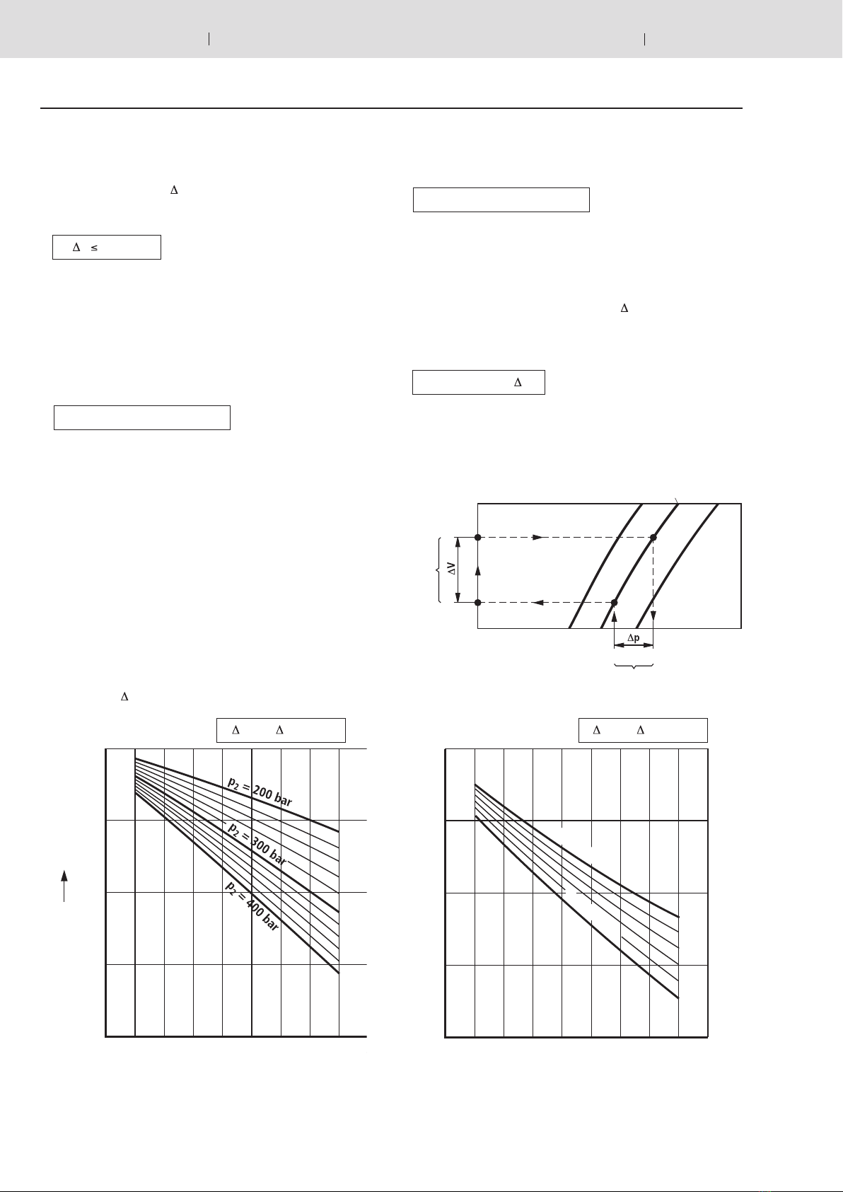
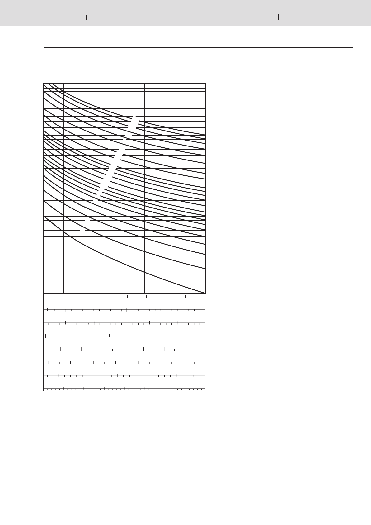
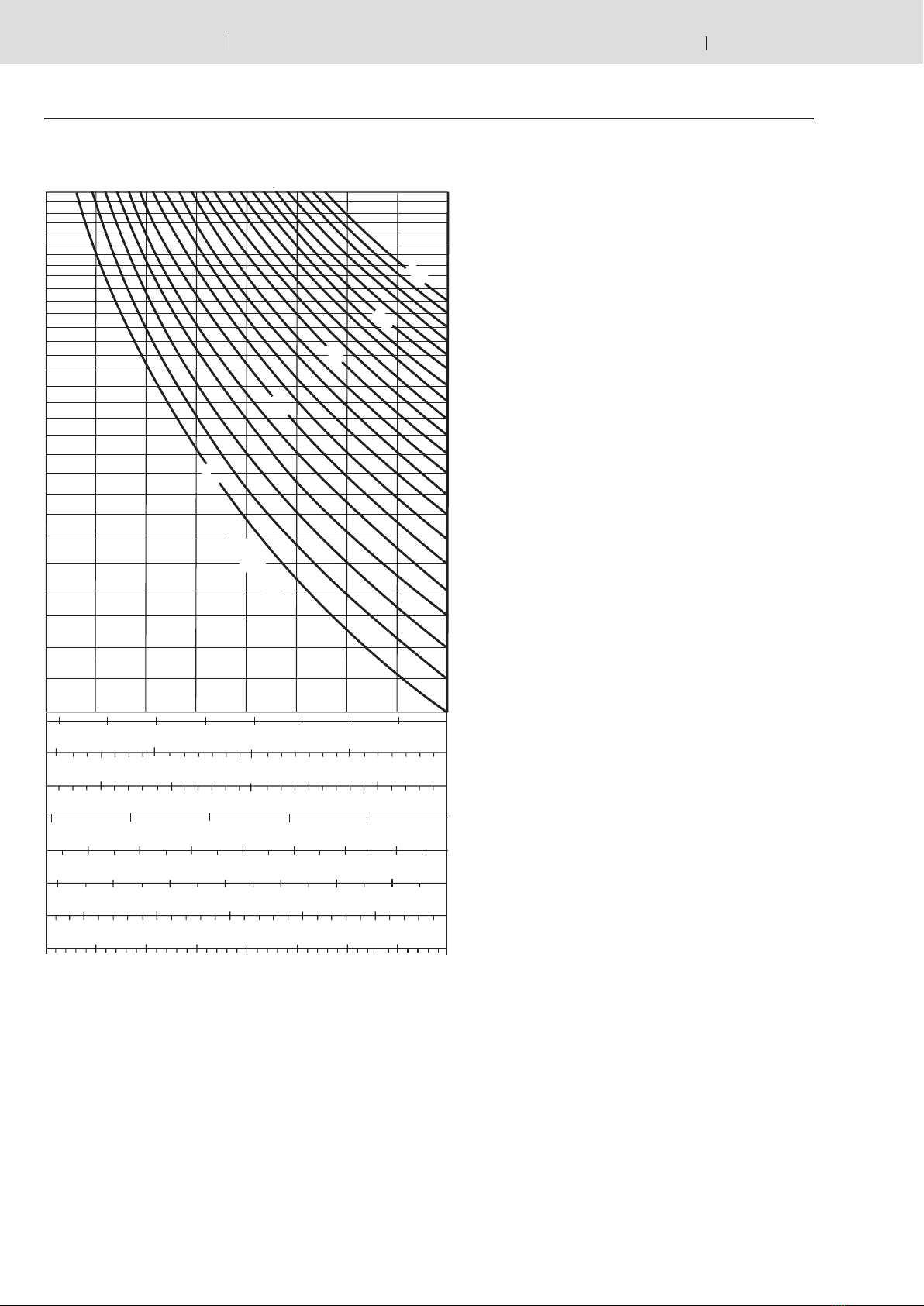
Calculation diagram
To allow a determination on the basis of a graphic rep-
resentation, the formulas (4.1) and (4.2) were translated
into diagrams on pages 7 to 10. Depending on the task at
hand, the available oil volume, the accumulator size or the
pressures can be established.
Available oil
volume
Gas charge pressure
Working pressure range
Correction factors Kiand Ka
Equations (4.1) and (4.2) are only valid for ideal gases. In
the characteristics of real gases, significant deviations can
be observed at operating pressures above 200 bar, which
must be taken into account by applying correction factors.
These are shown on the following diagrams. The correc-
tion factors which are to be multiplied by the ideal with-
drawal volume Vare within the range of 0.6 … 1.
Isothermal Vreal = Videal • KiVreal = Videal • Ka
Adiabatic
Vin l →
pin bar →
p1/ p2→
Ki→
Ka→
p1/ p2→