TiePie Handyscope HS5 series User manual

Handyscope HS5
User manual
TiePie engineering

ATTENTION!
Measuring directly on the line voltage can be very dangerous.
The outside of the BNC connectors at the Handyscope HS5 are
connected with the ground of the computer. Use a good isolation
transformer or a differential probe when measuring at the line volt-
age or at grounded power supplies! A short-circuit current will
flow if the ground of the Handyscope HS5 is connected to a positive
voltage. This short-circuit current can damage both the Handyscope
HS5 and the computer.
Copyright c 2016 TiePie engineering.
All rights reserved.
Revision 2.14, January 2016
Despite the care taken for the compilation of this
user manual, TiePie engineering can not be held
responsible for any damage resulting from errors
that may appear in this manual.

Contents
1 Safety 1
2 Declaration of conformity 3
3 Introduction 5
3.1 Sampling ........................ 7
3.2 Sample frequency .................... 8
3.2.1 Aliasing ..................... 9
3.3 Digitizing ........................ 10
3.4 Signal coupling ..................... 11
3.5 Probe compensation .................. 12
4 Driver installation 15
4.1 Introduction ....................... 15
4.2 Where to find the driver setup ............ 15
4.3 Executing the installation utility ........... 15
5 Hardware installation 21
5.1 Power the instrument ................. 21
5.1.1 External power ................. 21
5.2 Connect the instrument to the computer ....... 22
5.2.1 Found New Hardware Wizard ......... 22
5.3 Plug into a different USB port ............ 23
5.4 Operating conditions .................. 23
6 Combining instruments 25
7 Front panel 27
7.1 CH1 and CH2 input connectors ............ 27
7.2 AWG output connector ................ 27
7.3 Power indicator ..................... 27
8 Rear panel 29
8.1 Power .......................... 29
8.1.1 Power adapter ................. 30
8.1.2 USB power cable ................ 30
8.2 USB ........................... 31
8.3 Extension Connector .................. 31
Contents I

8.4 AUX I/O ........................ 32
9 Specifications 33
9.1 Acquisition system ................... 33
9.2 Acquisition system (continued) ............ 34
9.3 Trigger system ..................... 35
9.4 Arbitrary Waveform Generator ............ 36
9.5 Power .......................... 39
9.6 Multi-instrument synchronization ........... 39
9.7 Physical ......................... 39
9.8 I/O connectors ..................... 39
9.9 Interface ......................... 39
9.10 System requirements .................. 40
9.11 Environmental conditions ............... 40
9.12 Certifications and Compliances ............ 40
9.13 Probes .......................... 41
9.14 Package contents .................... 41
II

Safety 1
When working with electricity, no instrument can guaran-
tee complete safety. It is the responsibility of the person
who works with the instrument to operate it in a safe way.
Maximum security is achieved by selecting the proper in-
struments and following safe working procedures. Safe
working tips are given below:
•Always work according (local) regulations.
•Work on installations with voltages higher than 25 VAC or
60 VDC should only be performed by qualified personnel.
•Avoid working alone.
•Observe all indications on the Handyscope HS5 before con-
necting any wiring
•Check the probes/test leads for damages. Do not use them
if they are damaged
•Take care when measuring at voltages higher than 25 VAC or
60 VDC.
•Do not operate the equipment in an explosive atmosphere or
in the presence of flammable gases or fumes.
•Do not use the equipment if it does not operate properly.
Have the equipment inspected by qualified service personal.
If necessary, return the equipment to TiePie engineering for
service and repair to ensure that safety features are main-
tained.
•Measuring directly on the line voltage can be very danger-
ous. The outside of the BNC connectors at the Handy-
scope HS5 are connected with the ground of the computer.
Use a good isolation transformer or a differential probe when
measuring at the line voltage or at grounded power sup-
plies! A short-circuit current will flow if the ground of the
Handyscope HS5 is connected to a positive voltage. This
short-circuit current can damage both the Handyscope HS5
and the computer.
Safety 1

2Chapter 1

Declaration of conformity 2
TiePie engineering
Koperslagersstraat 37
8601 WL Sneek
The Netherlands
EC Declaration of conformity
We declare, on our own responsibility, that the product
Handyscope HS5-540(XM/S/XMS)
Handyscope HS5-530(XM/S/XMS)
Handyscope HS5-220(XM/S/XMS)
Handyscope HS5-110(XM/S/XMS)
Handyscope HS5-055(XM/S/XMS)
for which this declaration is valid, is in compliance with
EN 55011:2009/A1:2010 IEC 61000-6-1/EN 61000-6-1:2007
EN 55022:2006/A1:2007 IEC 61000-6-3/EN 61000-6-3:2007
according the conditions of the EMC standard 2004/108/EC
and also with
Canada: ICES-001:2004 Australia/New Zealand: AS/NZS
Sneek, 29-5-2012
ir. A.P.W.M. Poelsma
Declaration of conformity 3

Environmental considerations
This section provides information about the environmental impact
of the Handyscope HS5.
Handyscope HS5 end-of-life handling
Production of the Handyscope HS5 required the extraction and use
of natural resources. The equipment may contain substances that
could be harmful to the environment or human health if improperly
handled at the Handyscope HS5’s end of life.
In order to avoid release of such substances into the environment
and to reduce the use of natural resources, recycle the Handyscope
HS5 in an appropriate system that will ensure that most of the
materials are reused or recycled appropriately.
The symbol shown below indicates that the Handyscope HS5
complies with the European Union’s requirements according to Di-
rective 2002/96/EC on waste electrical and electronic equipment
(WEEE).
Restriction of Hazardous Substances
The Handyscope HS5 has been classified as Monitoring and Con-
trol equipment, and is outside the scope of the 2002/95/EC RoHS
Directive.
4Chapter 2

Introduction 3
Before using the Handyscope HS5 first read chapter 1about
safety.
Many technicians investigate electrical signals. Though the
measurement may not be electrical, the physical variable is of-
ten converted to an electrical signal, with a special transducer.
Common transducers are accelerometers, pressure probes, current
clamps and temperature probes. The advantages of converting the
physical parameters to electrical signals are large, since many in-
struments for examining electrical signals are available.
The Handyscope HS5 is a portable two channel measuring in-
strument with Arbitrary Waveform Generator. The Handyscope
HS5 is available in several models with different maximum sam-
pling frequencies: 50 MS/s, 100 MS/s, 200 MS/s or 500 MS/s.
The native resolutions are 8, 12 and 14 bits and a user selectable
resolution of 16 bits is available too, with adjusted maximum sam-
pling frequencies:
Handyscope HS5 Channels Resolution
8 / 12 bit 14 bit 16 bit
Model 540 CH1 500 MS/s 100 MS/s 6.25 MS/s
CH1+CH2 200 MS/s
Model 530 CH1 500 MS/s 100 MS/s 6.25 MS/s
CH1+CH2 200 MS/s
Model 220 CH1 200 MS/s 50 MS/s 3.125 MS/s
CH1+CH2 100 MS/s
Model 110 CH1 100 MS/s 20 MS/s 1.25 MS/s
CH1+CH2 50 MS/s
Model 055 CH1 50 MS/s 10 MS/s 625 kS/s
CH1+CH2 20 MS/s
Table 3.1: Maximum sampling frequencies
Introduction 5

The Handyscope HS5 supports high speed continuous streaming
measurements. The maximum streaming rates are:
Handyscope HS5 Channels Resolution
8 bit 12/14 bit 16 bit
Model 540 CH1 40 MS/s 20 MS/s 6.25 MS/s
CH1+CH2 20 MS/s 10 MS/s
Model 530 CH1 40 MS/s 20 MS/s 6.25 MS/s
CH1+CH2 20 MS/s 10 MS/s
Model 220 CH1 20 MS/s 10 MS/s 3.125 MS/s
CH1+CH2 10 MS/s 5 MS/s
Model 110 CH1 10 MS/s 5 MS/s 1.25 MS/s
CH1+CH2 4 MS/s 2 MS/s
Model 055 CH1 4 MS/s 2 MS/s 625 kS/s
CH1+CH2 2 MS/s 1 MS/s
Table 3.2: Maximum streaming rates
The Handyscope HS5 is available with two memory configura-
tions, these are:
Memory Model 540 Model 530 Model 220 Model 110 Model 055
Standard model 128 KiS 128 KiS 128 KiS 128 KiS 128 KiS
Option XM 32 MiS 32 MiS 32 MiS 32 MiS 32 MiS
Table 3.3: Maximum record lengths per channel
Optionally available for the Handyscope HS5 are SureConnect
connection test and resistance measurement. SureConnect connec-
tion test tells you immediately whether your test probe or clip
actually makes electrical contact or not. No more doubt whether
your probe doesn’t make contact or there really is no signal. This
is useful when surfaces are oxidized and your probe cannot get a
good electrical contact. Simply activate the SureConnect and you
know whether there is contact or not. Also when back probing con-
nectors in confined places, SureConnect immediately shows whether
the probes make contact or not.
Models of the Handyscope HS5 with SureConnect come with re-
sistance measurement on all channels. Resistances up to 2 MOhm
can be measured directly. Resistance can be shown in meter dis-
plays and can also be plotted versus time in a graph, creating an
Ohm scope.
6Chapter 3

With the accompanying software the Handyscope HS5 can be
used as an oscilloscope, a spectrum analyzer, a true RMS voltmeter
or a transient recorder. All instruments measure by sampling the
input signals, digitizing the values, process them, save them and
display them.
3.1 Sampling
When sampling the input signal, samples are taken at fixed inter-
vals. At these intervals, the size of the input signal is converted to a
number. The accuracy of this number depends on the resolution of
the instrument. The higher the resolution, the smaller the voltage
steps in which the input range of the instrument is divided. The
acquired numbers can be used for various purposes, e.g. to create
a graph.
Figure 3.1: Sampling
The sine wave in figure 3.1 is sampled at the dot positions. By
connecting the adjacent samples, the original signal can be recon-
structed from the samples. You can see the result in figure 3.2.
Introduction 7

Figure 3.2: ”connecting” the samples
3.2 Sample frequency
The rate at which the samples are taken is called the sampling
frequency, the number of samples per second. A higher sampling
frequency corresponds to a shorter interval between the samples.
As is visible in figure 3.3, with a higher sampling frequency, the
original signal can be reconstructed much better from the measured
samples.
Figure 3.3: The effect of the sampling frequency
The sampling frequency must be higher than 2 times the high-
est frequency in the input signal. This is called the Nyquist fre-
quency. Theoretically it is possible to reconstruct the input signal
with more than 2 samples per period. In practice, 10 to 20 sam-
8Chapter 3

ples per period are recommended to be able to examine the signal
thoroughly.
3.2.1 Aliasing
When sampling an analog signal with a certain sampling frequency,
signals appear in the output with frequencies equal to the sum and
difference of the signal frequency and multiples of the sampling
frequency. For example, when the sampling frequency is 1000 Hz
and the signal frequency is 1250 Hz, the following signal frequencies
will be present in the output data:
Multiple of sampling frequency 1250 Hz signal -1250 Hz signal
...
-1000 -1000 + 1250 = 250 -1000 - 1250 = -2250
0 0 + 1250 = 1250 0 - 1250 = -1250
1000 1000 + 1250 = 2250 1000 - 1250 = -250
2000 2000 + 1250 = 3250 2000 - 1250 = 750
...
Table 3.4: Aliasing
As stated before, when sampling a signal, only frequencies lower
than half the sampling frequency can be reconstructed. In this
case the sampling frequency is 1000 Hz, so we can we only observe
signals with a frequency ranging from 0 to 500 Hz. This means
that from the resulting frequencies in the table, we can only see
the 250 Hz signal in the sampled data. This signal is called an
alias of the original signal.
If the sampling frequency is lower than twice the frequency of
the input signal, aliasing will occur. The following illustration
shows what happens.
Introduction 9

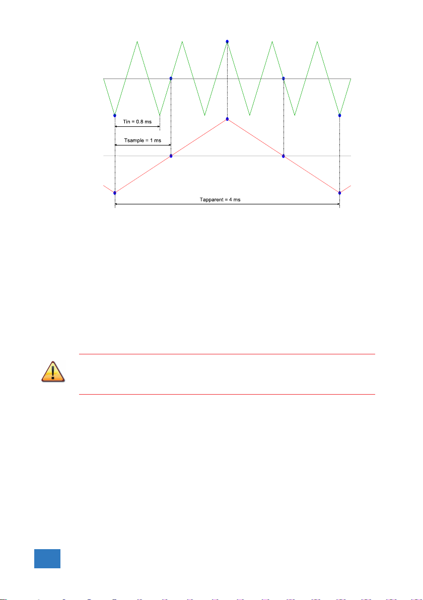
Figure 3.4: Aliasing
In figure 3.4, the green input signal (top) is a triangular signal
with a frequency of 1.25 kHz. The signal is sampled with a fre-
quency of 1 kHz. The corresponding sampling interval is 1/1000Hz
= 1ms. The positions at which the signal is sampled are depicted
with the blue dots. The red dotted signal (bottom) is the result
of the reconstruction. The period time of this triangular signal
appears to be 4 ms, which corresponds to an apparent frequency
(alias) of 250 Hz (1.25 kHz - 1 kHz).
To avoid aliasing, always start measuring at the highest sam-
pling frequency and lower the sampling frequency if required.
3.3 Digitizing
When digitizing the samples, the voltage at each sample time is
converted to a number. This is done by comparing the voltage
with a number of levels. The resulting number is the number cor-
responding to the level that is closest to the voltage. The number
of levels is determined by the resolution, according to the following
relation: LevelCount = 2Resolution.
10 Chapter 3

The higher the resolution, the more levels are available and
the more accurate the input signal can be reconstructed. In figure
3.5, the same signal is digitized, using two different amounts of
levels: 16 (4-bit) and 64 (6-bit).
Figure 3.5: The effect of the resolution
The Handyscope HS5 measures at e.g. 14 bit resolution (214=16384
levels). The smallest detectable voltage step depends on the input
range. This voltage can be calculated as:
V oltageStep =F ullInputRange/LevelCount
For example, the 200 mV range ranges from -200 mV to +200
mV, therefore the full range is 400 mV. This results in a smallest
detectable voltage step of 0.400V/16384 = 24.41 µV.
3.4 Signal coupling
The Handyscope HS5 has two different settings for the signal cou-
pling: AC and DC. In the setting DC, the signal is directly coupled
to the input circuit. All signal components available in the input
signal will arrive at the input circuit and will be measured.
In the setting AC, a capacitor will be placed between the input
connector and the input circuit. This capacitor will block all DC
components of the input signal and let all AC components pass
through. This can be used to remove a large DC component of the
input signal, to be able to measure a small AC component at high
resolution.
Introduction 11

When measuring DC signals, make sure to set the signal
coupling of the input to DC.
3.5 Probe compensation
The Handyscope HS5 is shipped with a probe for each input chan-
nel. These are 1x/10x selectable passive probes. This means that
the input signal is passed through directly or 10 times attenuated.
When using an oscilloscope probe in 1:1 the setting, the
bandwidth of the probe is only 6 MHz. The full bandwidth
of the probe is only obtained in the 1:10 setting
The x10 attenuation is achieved by means of an attenuation
network. This attenuation network has to be adjusted to the oscil-
loscope input circuitry, to guarantee frequency independency. This
is called the low frequency compensation. Each time a probe is
used on an other channel or an other oscilloscope, the probe must
be adjusted.
Therefore the probe is equiped with a setscrew, with which the
parallel capacity of the attenuation network can be altered. To
adjust the probe, switch the probe to the x10 and attach the probe
to a 1 kHz square wave signal. Then adjust the probe for a square
front corner on the square wave displayed. See also the following
illustrations.
12 Chapter 3

Figure 3.6: correct
Figure 3.7: under compensated
Figure 3.8: over compensated
Introduction 13

14 Chapter 3

Driver installation 4
Before connecting the Handyscope HS5 to the computer, the
drivers need to be installed.
4.1 Introduction
To operate a Handyscope HS5, a driver is required to interface
between the measurement software and the instrument. This driver
takes care of the low level communication between the computer
and the instrument, through USB. When the driver is not installed,
or an old, no longer compatible version of the driver is installed, the
software will not be able to operate the Handyscope HS5 properly
or even detect it at all.
The installation of the USB driver is done in a few steps. Firstly,
the driver has to be pre-installed by the driver setup program. This
makes sure that all required files are located where Windows can
find them. When the instrument is plugged in, Windows will detect
new hardware and install the required drivers.
4.2 Where to find the driver setup
The driver setup program and measurement software can be found
in the download section on TiePie engineering’s website and on the
CD-ROM that came with the instrument. It is recommended to
install the latest version of the software and USB driver from the
website. This will guarantee the latest features are included.
4.3 Executing the installation utility
To start the driver installation, execute the downloaded driver
setup program, or the one on the CD-ROM that came with the
instrument. The driver install utility can be used for a first time
Driver installation 15

installation of a driver on a system and also to update an existing
driver.
The screen shots in this description may differ from the ones
displayed on your computer, depending on the Windows version.
Figure 4.1: Driver install: step 1
When drivers were already installed, the install utility will re-
move them before installing the new driver. To remove the old
driver successfully, it is essential that the Handyscope HS5 is
disconnected from the computer prior to starting the driver install
utility. When the Handyscope HS5 is used with an external power
supply, this must be disconnected too.
16 Chapter 4