biochrom EZ Read 400 User manual

Technical Tip: Transferring quantitative data from ADAP to MS Excel Version 2.0
1
BIOCHROM EZ READ 400 MICROPLATE READER
TECH TIPS: USING A STANDARD CURVE TO PREDICT THE CONCENTRATIONS
OF UNKNOWNS
Data can be easily exported from ADAP Basic into Excel for analysis. Many laboratory experiments are
quantitative tests which use a standard curve to predict the concentration of unknown samples. This
technical tip guides the user from gathering and exporting data using ADAP into Excel in order to
determine unknown concentrations.
1. Connect instrument to a power source using the appropriate power cord and power supply. Switch
on instrument.
Check the user’s manual for important safety information.
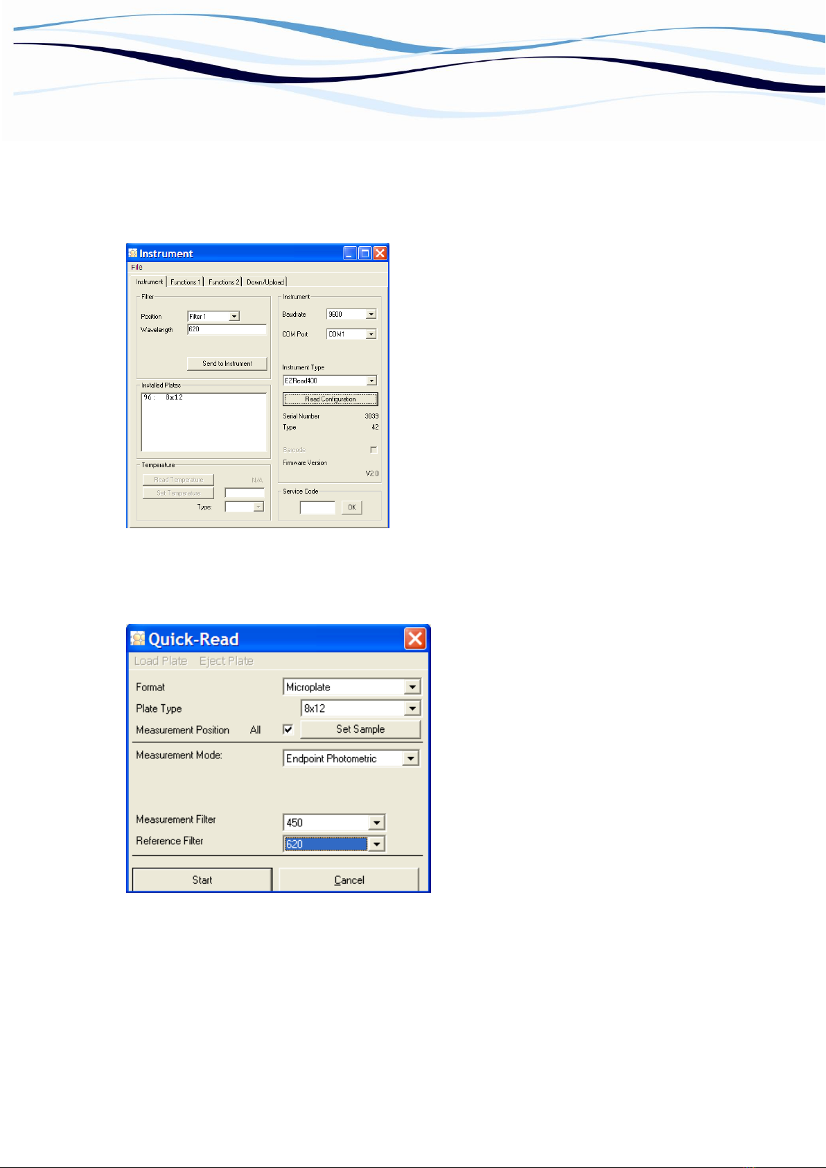
2. Connect the instrument to a PC: Ensure that you first have administrator rights for installing the
software and connecting the instrument to the PC for the first time. Connect to the PC to the
instrument using the USB port on the PC to the USB port on the back of the instrument using the
supplied USB A to B cable. Determine the communication port (COM) used by the instrument. In
the Start menu of the PC, go to Control Panel\System\Hardware\Device Manager\Ports to
determine the COM port used by the instrument. If you are unsure which COM port is being used,
please disconnect and connect the USB cable and observe which COM port reappears after re-
connecting to the PC.
Please Note: The instrument cannot connect to the PC if a COM port higher that 9 is used. If this is
the case please use the supplied COM port reassignment utilty to reassign the COM port to any
unused port from 1-9.
3. Insert the CD supplied with the instrument into the PC that will be used to control the instrument.
Install ADAP. Once the program is installed, open ADAP. ADAP will prompt for a user ID and
password. For the first time the program is used, enter the pre-set ID and passwords:
sadmin\sadmin.
4. Once logged as sadmin, the change password button will appear. Select this option to set specific
user IDs, passwords and administrative rights.
Figure 1 ADAP Login
Configure the login and users by entering in the user
name and password and the level of administrator rights.
Level 1 (user) can use ADAP for perform quick
measurements or use test definitions to acquire and
analyze data.
Level 2 (administrator) can perform all basic
measurements, create new test definitions for data
collection and analysis and can configure system and
instrument parameters.

Technical Tip: Transferring quantitative data from ADAP to MS Excel Version 2.0
2
Level 3 (system administrator) has the same privileges as levels 1 and 2 as well as the ability to add,
delete or edit users.
5. Select Setup>Instrument in the menu bar. A dialogue box will open:
Figure 2 Connect to the Instrument
In the Instrument tab, select
Baudrate: select Auto Sense
COM Port: select port as determined in step 2
Instrument Type: select EZ Read 400
Select File>Save to return to main menu and confirm the connection to the instrument.
6. To measure a plate:
Go to Reading/Quick or the R button in the menu bar.
Figure 3 Quick Read Dialogue Box
In the Quick-Read dialogue box:
Confirm that the correct format and plate
type are selected.
Select All in Measurement Position to
read the entire plate.
Select Endpoint Photometric for basic
readings using a measurement and
reference filter.
Select the measurement filter and the
reference filter from the drop-down
menu.
Note: It is important to use a reference filter to account for optical inference from the plate.
7. Place plate in the plate transporter. Select Start. Absorbance measurements will appear in the
open matrix in ADAP. When prompted, enter a plate ID.
8. Export the data. Ensure that absorbance measurements are visible in the open matrix. If not,
select the OD tab so that the absorbance data can be seen in the open matrix. In the menu bar,

Technical Tip: Transferring quantitative data from ADAP to MS Excel Version 2.0
3
select Options>Copy all data on to clipboard. Now open Excel. Select Paste or control (v) to paste
into the empty workbook. Data will paste as a matrix with filter wavelength, with time and date.
9. In a new Excel spreadsheet, layout the page with the plate layout and raw data:
Data Export
1
2
3
4
5
6
7
8
9
10
11
12
A
1.453
1.446
1.398
1.432
0.240
0.085
0.503
0.082
0.086
0.440
0.085
0.091
B
0.729
0.720
0.714
0.615
0.595
0.118
0.082
0.648
0.130
0.088
0.435
0.082
C
0.431
0.432
0.420
0.386
0.087
0.084
0.570
0.129
0.084
0.082
0.084
0.085
D
0.239
0.234
0.235
0.217
0.237
0.334
0.081
0.084
0.090
0.173
0.086
0.088
E
0.146
0.145
0.148
0.156
0.090
0.086
0.081
0.256
0.084
0.085
0.578
0.601
F
0.109
0.115
0.115
0.108
0.508
0.086
0.500
0.083
0.336
0.085
0.092
0.085
G
0.096
0.150
0.099
0.097
0.082
0.337
0.082
0.156
0.414
0.088
0.084
0.088
H
0.088
0.090
0.092
0.086
0.166
0.085
0.634
0.088
0.101
0.091
0.089
0.082
10. Determine the average absorbance of the blank wells and subtract this value from the remaining
wells:
Average Blank Absorbance:
B1
B2
B3
B4
Mean (OD)
0.088
0.09
0.092
0.086
0.089
Blank Corrected Absorbance:
1
2
3
4
5
6
7
8
9
10
11
12
A
1.364
1.357
1.309
1.343
0.151
-0.004
0.414
-0.007
-0.003
0.351
-0.004
0.002
B
0.640
0.631
0.625
0.526
0.506
0.029
-0.007
0.559
0.041
-0.001
0.346
-0.007
C
0.342
0.343
0.331
0.297
-0.002
-0.005
0.481
0.040
-0.005
-0.007
-0.005
-0.004
D
0.150
0.145
0.146
0.128
0.148
0.245
-0.008
-0.005
0.001
0.084
-0.003
-0.001
E
0.057
0.056
0.059
0.067
0.001
-0.003
-0.008
0.167
-0.005
-0.004
0.489
0.512
F
0.020
0.026
0.026
0.019
0.419
-0.003
0.411
-0.006
0.247
-0.004
0.003
-0.004
G
0.007
0.061
0.010
0.008
-0.007
0.248
-0.007
0.067
0.325
-0.001
-0.005
-0.001
H
-0.001
0.001
0.003
-0.003
0.077
-0.004
0.545
-0.001
0.012
0.002
0.000
-0.007
Plate Layout
1
2
3
4
5
6
7
8
9
10
11
12
A
S1
S1
S1
S1
1
9
17
25
33
41
49
57
Standards
B
S2
S3
S4
S5
2
10
18
26
34
42
50
58
Blank
C
S3
S4
S5
S6
3
11
19
27
35
43
51
59
Samples
D
S4
S4
S4
S4
4
12
20
28
36
44
52
60
E
S5
S5
S5
S5
5
13
21
29
37
45
53
61
F
S6
S6
S6
S6
6
14
22
30
38
46
54
62
G
S7
S7
S7
S7
7
15
23
31
39
47
55
63
H
Blank
Blank
Blank
Blank
8
16
24
32
40
48
56
64

Technical Tip: Transferring quantitative data from ADAP to MS Excel Version 2.0
4
11. Next, compile a table of the blank corrected absorbance values of the standards:
Well
Label
Compound
X
(g/mL)
1
2
3
4
Mean
(OD)
Standard
Deviation
(OD)
Coefficient
of
Variation
(%)
S1
100.00
1.364
1.357
1.309
1.343
1.343
0.030
2.23%
S2
50
0.640
0.631
0.625
0.526
0.632
0.008
1.19%
S3
25.00
0.342
0.343
0.331
0.297
0.339
0.007
1.97%
S4
12.50
0.150
0.145
0.146
0.128
0.147
0.003
1.80%
S5
6.25
0.057
0.056
0.059
0.067
0.057
0.002
2.66%
S6
3.13
0.020
0.026
0.026
0.019
0.024
0.003
14.43%
S7
1.56
0.007
0.061
0.010
0.008
0.026
0.030
116.72%
For each standard, calculate the mean or average value, standard deviation and coefficient of variation
using the following formulas in Excel:
Mean Standard 1 (S1): =AVERAGE(wells A1, A2, A3 and A4)
Standard Deviation S1: =STDEV(wells A1, A2, A3 and A4)
Coefficient of Variation (%CV) =standard deviation/mean*100%
The %CV is a useful metric for determining the reliability of the data. Typically, %CV of <5% suggests
that the data is reliable (this assumption is assay type dependent). Thus the mean absorbance values
of S6 and S7 will not be included in the standard curve because the %CV is >5% (14.4% and 116.7%
respectively).
12. Plot the mean absorbance values of standards S1 –S5 as a function of the known concentrations as a
x-y scatter plot:
Fit a linear regression trend line to the data by selecting trend line in the chart layout menu. The
example data conforms to the linear trend as represented by the R2value: 0.9989 or 99.89%.Thus the
equation of the linear regression trend line can be used to determine the concentration of samples
y = 0.0136x - 0.0231
R² = 0.9989
0.000
0.200
0.400
0.600
0.800
1.000
1.200
1.400
0.00 20.00 40.00 60.00 80.00 100.00
Absorbance @ 450 nm
Concentration (ug/mL)
Absorbance vs Concentration of Compound X
Compound X
Linear
(Compound X)

Technical Tip: Transferring quantitative data from ADAP to MS Excel Version 2.0
5
from their absorbance values. The standard deviation from the mean absorbance values were used to
plot error bars to the data points
Please note: The standard deviation can be used to fit y-error bars to the data (as shown above).
Please note: Other curve fitting algorithms may be more appropriate to your data such as 4-parameter
fit, cubic spline or polynomial regression.
13. The equation of the line is then used to calculate the concentration of the samples by solving for x and
inputting the blank-corrected absorbance for the y value:
Concentrations (ug/mL)
1
2
3
4
5
6
7
8
9
10
11
12
A
101.99
101.48
97.95
100.45
12.80
1.40
32.14
1.18
1.48
27.51
1.40
1.85
B
48.76
48.10
47.65
40.38
38.90
3.83
1.18
42.80
4.71
1.63
27.14
1.18
C
26.85
26.92
26.04
23.54
1.55
1.33
37.07
4.64
1.33
1.18
1.33
1.40
D
12.73
12.36
12.43
11.11
12.58
19.71
1.11
1.33
1.77
7.88
1.48
1.63
E
5.89
5.82
6.04
6.63
1.77
1.48
1.11
13.98
1.33
1.40
37.65
39.35
F
3.17
3.61
3.61
3.10
32.51
1.48
31.92
1.26
19.86
1.40
1.92
1.40
G
2.21
6.18
2.43
2.29
1.18
19.93
1.18
6.63
25.60
1.63
1.33
1.63
H
1.63
1.77
1.92
1.48
7.36
1.40
41.77
1.63
2.58
1.85
1.70
1.18
These concentration values are based on the standard curve, thus only concentrations that are >100
ug/mL or <3.13 ug/mL are considered valid; all other values are disregarded. A small amount of
extrapolation may be acceptable depending on the linear range of the instrument and the linear range
of the assay.