Hameg HM1500-2 User manual

150 MHz
Analog Oscilloscope
HM1500-2
Manual
English
99 Washington Street
Melrose, MA 02176
Fax [phone]
TestEquipmentDepot.com

2Subject to change without notice
Hersteller HAMEG Instruments GmbH KONFORMITÄTSERKLÄRUNG
Manufacturer Industriestraße 6 DECLARATION OF CONFORMITY
Fabricant D-63533 Mainhausen DECLARATION DE CONFORMITE
General information regarding the CE marking
HAMEG instruments fulfill the regulations of the EMC directive. The
conformity test made by HAMEG is based on the actual generic- and
product standards. In cases where different limit values are applicable,
HAMEG applies the severer standard. For emission the limits for
residential, commercial and light industry are applied. Regarding the
immunity (susceptibility) the limits for industrial environment have
been used.
The measuring- and data lines of the instrument have much influence
on emmission and immunity and therefore on meeting the acceptance
limits. For different applications the lines and/or cables used may
be different. For measurement operation the following hints and
conditions regarding emission and immunity should be observed:
1. Data cables
For the connection between instruments respectively their interfaces
and external devices, (computer, printer etc.) sufficiently screened
cables must be used. Without a special instruction in the manual for
a reduced cable length, the maximum cable length of a dataline must
be less than 3 meters and not be used outside buildings. If an interface
has several connectors only one connector must have a connection
to a cable.
Basically interconnections must have a double screening. For IEEE-bus
purposes the double screened cables HZ73 and HZ72L from HAMEG
are suitable.
2. Signal cables
Basically test leads for signal interconnection between test point and
instrument should be as short as possible. Without instruction in the
manual for a shorter length, signal lines must be less than 3 meters
and not be used outside buildings.
Signal lines must screened (coaxial cable - RG58/U). A proper ground
connection is required. In combination with signal generators double
screened cables (RG223/U, RG214/U) must be used.
Die HAMEG Instruments GmbH bescheinigt die Konformität für das Produkt
The HAMEG Instruments GmbH herewith declares conformity of the product
HAMEG Instruments GmbH déclare la conformite du produit
Bezeichnung / Product name / Designation:
Oszilloskop
Oscilloscope
Oscilloscope
Typ / Type / Type: HM1500-2
mit / with / avec: –
Optionen / Options / Options: –
mit den folgenden Bestimmungen / with applicable regulations / avec les
directives suivantes
EMV Richtlinie 89/336/EWG ergänzt durch 91/263/EWG, 92/31/EWG
EMC Directive 89/336/EEC amended by 91/263/EWG, 92/31/EEC
Directive EMC 89/336/CEE amendée par 91/263/EWG, 92/31/CEE
Niederspannungsrichtlinie 73/23/EWG ergänzt durch 93/68/EWG
Low-Voltage Equipment Directive 73/23/EEC amended by 93/68/EEC
Directive des equipements basse tension 73/23/CEE amendée par 93/68/CEE
Angewendete harmonisierte Normen / Harmonized standards applied / Normes
harmonisées utilisées:
Sicherheit / Safety / Sécurité: EN 61010-1:2001 (IEC 61010-1:2001)
Überspannungskategorie / Overvoltage category / Catégorie de surtension: II
Verschmutzungsgrad / Degree of pollution / Degré de pollution: 2
Elektromagnetische Verträglichkeit / Electromagnetic compatibility /
Compatibilité électromagnétique
EN 61326-1/A1 Störaussendung / Radiation / Emission:
Tabelle / table / tableau 4; Klasse / Class / Classe B.
Störfestigkeit / Immunity / Imunitée:Tabelle / table / tableau A1.
EN 61000-3-2/A14 Oberschwingungsströme / Harmonic current emissions /
Émissions de courant harmonique:
Klasse / Class / Classe D.
EN 61000-3-3 Spannungsschwankungen u. Flicker / Voltage fluctuations and flicker /
Fluctuations de tension et du flicker.
Datum /Date /Date
01. 06. 2007
Unterschrift / Signature / Signatur
Holger Asmussen
Manager
3. Influence on measuring instruments
Under the presence of strong high frequency electric or magnetic fields,
even with careful setup of the measuring equipment an influence of
such signals is unavoidable.
This will not cause damage or put the instrument out of operation. Small
deviations of the measuring value (reading) exceeding the instruments
specifications may result from such conditions in individual cases.
4. RF immunity of oscilloscopes.
4.1 Electromagnetic RF field
The influence of electric and magnetic RF fields may become visible
(e.g. RF superimposed), if the field intensity is high. In most cases
the coupling into the oscilloscope takes place via the device under
test, mains/line supply, test leads, control cables and/or radiation.
The device under test as well as the oscilloscope may be effected by
such fields.
Although the interior of the oscilloscope is screened by the cabinet,
direct radiation can occur via the CRT gap. As the bandwidth of
each amplifier stage is higher than the total –3dB bandwidth of the
oscilloscope, the influence RF fields of even higher frequencies may
be noticeable.
4.2 Electrical fast transients / electrostatic discharge
Electrical fast transient signals (burst) may be coupled into the
oscilloscope directly via the mains/line supply, or indirectly via test
leads and/or control cables. Due to the high trigger and input sensitivity
of the oscilloscopes, such normally high signals may effect the trigger
unit and/or may become visible on the CRT, which is unavoidable.
These effects can also be caused by direct or indirect electrostatic
discharge.
HAMEG Instruments GmbH

3
Subject to change without notice
Contents
General information regarding the CE marking 2
150 MHz 2-Chanel Analog Oscilloscope HM1500-2 4
Specifications 5
Important hints 6
List of symbols used: 6
Positioning the instrument 6
Safety 6
Proper operation 6
CAT I 6
Environment of use 6
Environmental conditions 7
Warranty and repair 7
Maintenance 7
Line voltage 7
Front Panel Elements – Brief Description 8
Basic signal measurement 10
Signals which can be measured 10
Amplitude of signals 10
Values of a sine wave signal 10
DC and AC components of an input signal 11
Timing relationships 11
Connection of signals 11
First time operation and initial adjustments 12
Trace rotation TR 12
Probe adjustment and use 12
1 kHz adjustment 12
1 MHz adjustment 13
Operating modes of the vertical amplifier 13
XY operation 14
Phase measurements with Lissajous figures 14
Measurement of phase differences in dual
channel Yt mode 14
Measurement of amplitude modulation 15
Triggering and time base 16
Automatic peak triggering (MODE menu) 16
Normal trigger mode (See menu MODE) 16
Slope selection (Menu FILTER) 16
Trigger coupling (Menu: FILTER) 16
Video (tv triggering) 17
Frame sync pulse triggering 17
Line sync pulse triggering 17
LINE trigger 17
Alternate trigger 17
External triggering 18
Indication of triggered operation (TRIG’D LED) 18
Hold-off time adjustment 18
Time base B (2nd time base). Delaying,
Delayed Sweep 18
Alternate sweep 19
AUTOSET 19
Component tester 20
Data transfer 21
General information concerning MENU 22
Controls and Readout 23

4Subject to change without notice
HM1500-2
Two Channels with deflection coefficients of 1 mV – 20 V/cm
Low Noise Measuring Amplifiers with high pulse fidelity
Two Time Bases: 0.5 s – 5 ns/cm and 20 ms – 5 ns/cm
Videotrigger: Odd and even frames, line selection (525/60 and
625/50 standard)
200 MHz 6-Digit Frequency Counter, Cursor and Automatic
Measurement
14 kV high writing speed CRT, Readout, Autoset, Delay Line,
no Fan
Save/Recall Memories for instrument settings
Help Function, Multilingual Menu
150 MHz Analog Oscilloscope
HM1500-2
Lissajous Figure (XY Mode)
199.994 MHz Sine Wave
Signal, measured with
internal frequency counter.
Excellent dynamic range
characteristics demonstra-
ted with a 150 MHz signal

5
Subject to change without notice
Specifications
150 MHz Analog Oszilloscope HM1500-2
Valid at 23 °C after a 30 minute warm-up period
Vertical Deflection
Channels: 2
Operating Modes: CH 1 or CH 2 separate,
DUAL (CH 1 and CH 2 alternate or chopped),
Addition
X in XY-Mode: CH 1
Invert: CH 1, CH 2
Bandwidth (-3dB): 2 x 0 - 150 MHz
Rise time: ‹2.3ns
Overshoot: max. 1 %
Bandwith limiting (selectable):about 20 MHz (5 mV/cm - 20 V/cm)
Deflection Coefficients(CH 1,2):14 calibrated steps
1 mV – 2 mV/cm: ± 5 % (0 - 10 MHz (-3 dB))
5 mV – 20 V/cm: ± 3 % (1-2-5 sequence)
variable (uncalibrated) › 2.5 :1 to › 50 V/cm
Inputs CH 1, 2:
Input Impedance: 1 MΩ II 15 pF
Coupling: DC, AC, GND (ground)
Max. Input Voltage: 400 V (DC + peak AC)
Y Delay Line: 70 ns
Measuring Circuits: Measuring Category I
Auxiliary input:
Function (selectable): Extern Trigger, Z (unblank)
Coupling: AC, DC
Max. input voltage: 100 V (DC + peak AC)
Triggering
Automatic (Peak to Peak):
Min. signal height: 5mm
Frequency range: 10 Hz - 250 MHz
Level control range: from Peak- to Peak+
Normal (without peak)
Min. signal height: 5mm
Frequency range: 0 - 250 MHz
Level control range: –10 cm to +10 cm
Operating modes: Slope/Video
Slope: positive, negative, both
Sources: CH 1, CH 2, alt. CH 1/2 (≥8 mm), Line, Ext.
Coupling: AC: 10 Hz-250 MHz
DC: 0-250 MHz
HF: 30 kHz–250 MHz
LF: 0-5kHz
Noise Rej. switchable
Video: pos./neg. Sync. Impulse
Standards: 525 Line/60 Hz Systems
625 Line/50 Hz Systems
Field: even/odd/both
Line: all/line number selectable
Source: CH 1, CH 2, Ext.
Indicator for trigger action: LED
External Trigger via: Auxiliary Input (0.3 Vpp, 150 MHz)
Coupling: AC, DC
Max. input voltage: 100 V (DC +peak AC)
2nd Trigger
Min. signal height: 5mm
Frequency range: 0 – 250 MHz
Coupling: DC
Level control range: -10 cm to +10 cm
Horizontal Deflection
Operating modes: A, ALT (alternating A/B), B
Time base A: 0.5 s/cm - 50 ns/cm (1-2-5 sequence)
Time base B: 20 ms/cm - 50 ns/cm (1-2-5 sequence)
Accuracy A and B: ±3%
X Magnification x10: to 5 ns/cm
Accuracy X x10: ±5%
Variable time base A/B: cont. 1:2.5
Hold Off time: var. 1:10 LED-Indication
Bandwidth X-Amplifier: 0 – 3 MHz (-3 dB)
XY phase shift ‹ 3°: ‹ 220 kHz
Operation/Measuring/Interfaces
Operation: Autoset, Menu and help functions (multilingual)
Save/Recall (instrument parameter settings): 9
Signal display: max. 4 traces
CH 1, 2 (Time Base A) in combination with
CH 1, 2 (Time Base B)
Frequency counter:
6 digit resolution: ›1 MHz – 250 MHz
5 digit resolution: 0.5 Hz – 1 MHz
Accuracy 50 ppm
Auto Measurements: Frequency, Period, Vdc, Vpp, Vp+, Vp-
Cursor Measurements: Δt, 1/Δt (f), tr, ΔV, V to GND, ratio X, ratio Y
Resolution Readout/Cursor: 1000 x 2000 Pts
Interfaces (plug-in): RS-232 (HO710),
Optional: Dual-Interface USB/RS232, IEEE-488 (GBIP)
Dual-Interface Ethernet/USB
Display
CRT: D14-375GH
Display area (with graticule): 8 cm x 10 cm
Acceleration voltage: ca. 14 kV
General Information
Component tester:
Test voltage: approx. 7 Vrms (open circuit), approx. 50Hz
Test current: max. 7 mArms (short circuit)
Reference Potential: Ground (safety earth)
Probe ADJ Output: 1 kHz/1 MHz square wave signal
0.2 Vpp (tr ‹ 4 ns)
Trace rotation: electronic
Line voltage: 105 – 253 V, 50/60 Hz ±10 %, CAT II
Power consumption: 37 Watt at 230V, 50 Hz
Protective system: Safety class I (EN61010-1)
Weight: 5.6 kg
Cabinet (W x H x D): 285 x 125 x 380 mm
Ambient temperature: 0° C ...+40° C
Accessories supplied: Line cord, Operating manual, 2 Probes 10:1 with
attenuation ID
Optional accessories:
HO720 Dual-Interface RS-232/USB
HO730 Dual-Interface Ethernet/USB
HO740 Interface IEEE-488 (GPIB)
HZ70 Opto-Interface (with optical fiber cable)
Test Equipment Depot - 800.517.8431 - 99 Washington Street Melrose, MA 02176
FAX [phone] - TestEquipmentDepot.com

6Subject to change without notice
Safe operation may be endangered if any of the following
was noticed:
– in case of visible damage.
– in case loose parts were noticed
– if it does not function any more.
– after prolonged storage under unfavourable conditions (e.g.
like in the open or in moist atmosphere).
– after any improper transport (e.g. insufficient packing not
conforming to the minimum standards of post, rail or trans-
port firm)
Proper operation
Please note: This instrument is only destined for use by person-
nel well instructed and familiar with the dangers of electrical
measurements.
For safety reasons the oscilloscope may only be operated from
mains outlets with safety ground connector. It is prohibited
to separate the safety ground connection. The plug must be
inserted prior to connecting any signals.
CAT I
This oscilloscope is destined for measurements in circuits not
connected to the mains or only indirectly. Direct measurements,
Important hints
Please check the instrument for mechanical damage or loose
parts immediately after unpacking. In case of damage we advise
to contact the sender. Do not operate.
List of symbols used:
Consult the manual High voltage
STOP
Important note Ground
Positioning the instrument
As can be seen from the figures, the handle can be set into
different positions:
A = carrying
B = handle removal and horizontal carrying
C = horizontal operating
D and E = operating at different angles
F = handle removal
T = shipping (handle unlocked)
STOP
Attention!
When changing the handle position, the instrument
must be placed so that it can not fall (e.g. placed
on a table). Then the handle locking knobs must be
simultaneously pulled outwards and rotated to the
required position. Without pulling the locking knobs
they will latch in into the next locking position.
Handle mounting/dismounting
The handle can be removed by pulling it out further, depending
on the instrument model in position B or F.
Safety
The instrument fulfils the VDE 0411 part 1 regulations for elec-
trical measuring, control and laboratory instruments and was
manufactured and tested accordingly. It left the factory in perfect
safe condition. Hence it also corresponds to European Standard
EN 61010-1 respectively International Standard IEC 1010-1. In
order to maintain this condition and to ensure safe operation the
user is required to observe the warnings and other directions
for use in this manual. Housing, chassis as well as all measu-
ring terminals are connected to safety ground of the mains.
All accessible metal parts were tested against the mains with
2200 VDC. The instrument conforms to safety class I.
The oscilloscope may only be operated from mains outlets with
a safety ground connector. The plug has to be installed prior to
connecting any signals. It is prohibited to separate the safety
ground connection.
Most electron tubes generate X-rays; the ion dose rate of this in-
strument remains well below the 36 pA/kg permitted by law.
In case safe operation may not be guaranteed do not use the
instrument any more and lock it away in a secure place.
Important hints
A
A
B
B
C
C
D
D
E
E
T
F
PUkT
PUkT
PUk PUk PUk PUk PUk PUk
PUkT PUkT
PUkT
PUkT
PUkT
HGOPFFD
PUkT
HGOFFD
PUOPFGkT
PUkT
PUkTKl
15pF
max
400Vp
PUOPFGkT
PUOPFGkT
PUOPFGkT
PUOPFGkT
PGkT PUOPFGkT
PUOPFGkT PFGkT
PUOPFGkTPUOPFGkT
PUOPFGkT PUOPFGkT
PUOPFGkT
HAMEG
PUOPFGkT
PUOPFGkT
PUOPFGkT
ANALOG
DIGITAL
MIXED SIGNAL
COMBISCOPE
HM1508
1 GSa · 1MB
150 MHz
PUOGkT
VOLTS/DIVV
HGOPFFD
VOLTS/DIVV
HGOPFFD
VOLTS/DIVV
HGOPFFD
PUkT
HGOPFFD
PUkT
HGOPFFD
PUkT
PUkT
PUkT
PUkT
PUkT
PUkT PUkT
PUkTKl
15pF
max
400Vp
PUOPFGkT
INPUTS
PUOPF
PUOPF
PUOPF
PUOPF PUOPF
C O M B I S C O P E
B
T
T

7
Subject to change without notice
Type of fuse:
Size 5 x 20 mm; 250V~, C;
IEC 127, Bl. III; DIN 41 662
(or DIN 41 571, Bl. 3).
Cut off: slow blow (T) 0,8A.
i.e. with a galvanic connection to circuits corresponding to the
categories II, III, or IV are prohibited!
The measuring circuits are considered not connected to the
mains if a suitable isolation transformer fulfilling safety class
II is used. Measurements on the mains are also possible if
suitable probes like current probes are used which fulfil the
safety class II. The measurement category of such probes must
be checked and observed.
Measurement categories
The measurement categories were derived corresponding to
the distance from the power station and the transients to be
expected hence. Transients are short, very fast voltage or cur-
rent excursions which may be periodic or not.
Measurement CAT IV:
Measurements close to the power station, e.g. on electricity
meters
Measurement CAT III:
Measurements in the interior of buildings (power distribution
installations, mains outlets, motors which are permanently
installed).
Measurement CAT II:
Measurements in circuits directly connected to the mains
(household appliances, power tools etc).
Environment of use.
The oscilloscope is destined for operation in industrial, business,
manufacturing, and living sites.
Environmental conditions
Operating ambient temperature: 0 to + 40 degrees C. During
transport or storage the temperature may be –20 to +55 de-
grees C.
Please note that after exposure to such temperatures or in case
of condensation proper time must be allowed until the instru-
ment has reached the permissible range of 0 to + 40 degrees
respectively until the condensation has evaporated before it may
be turned on! Ordinarily this will be the case after 2 hours. The
oscilloscope is destined for use in clean and dry environments.
Do not operate in dusty or chemically aggressive atmosphere
or if there is danger of explosion.
The operating position may be any, however, sufficient ventila-
tion must be ensured (convection cooling). Prolonged operation
requires the horizontal or inclined position.
STOP
Do not obstruct the ventilation holes!
Specifications are valid after a 20 minute warm-up period
between 15 and 30 degr. C. Specifications without tolerances
are average values.
Warranty and repair
HAMEG instruments are subjected to a rigorous quality control.
Prior to shipment each instrument will be burnt in for 10 hours.
Intermittent operation will produce nearly all early failures.
After burn in, a final functional and quality test is performed to
Important hints
check all operating modes and fulfilment of specifications. The
latter is performed with test equipment traceable to national
measurement standards.
Statutory warranty regulations apply in the country where the
HAMEG product was purchased. In case of complaints please
contact the dealer who supplied your HAMEG product.
Maintenance
Clean the outer shell using a dust brush in regular intervals.
Dirt can be removed from housing, handle, all metal and plastic
parts using a cloth moistened with water and 1 % detergent.
Greasy dirt may be removed with benzene (petroleum ether) or
alcohol, there after wipe the surfaces with a dry cloth. Plastic
parts should be treated with an antistatic solution destined
for such parts. No fluid may enter the instrument. Do not use
other cleansing agents as they may adversely affect the plastic
or lacquered surfaces.
Line voltage
The instrument has a wide range power supply from 105 to 253
V, 50 or 60 Hz ±10%. There is hence no line voltage selector.
The line fuse is accessible on the rear panel and part of the line
input connector. Prior to exchanging a fuse the line cord must
be pulled out. Exchange is only allowed if the fuse holder is
undamaged, it can be taken out using a screwdriver put into the
slot. The fuse can be pushed out of its holder and exchanged.
The holder with the new fuse can then be pushed back in place
against the spring. It is prohibited to ”repair“ blown fuses or to
bridge the fuse. Any damages incurred by such measures will
void the warranty.

8Subject to change without notice
Front Panel Elements – Brief Description
1
POWER (pushbutton) 23
Turns scope on and off.
2
INTENS (knob) 23
Intensity for trace and readout brightness, focus, trace
rotation and other control functions.
3
FOCUS, TRACE, MENU (pushbutton) 23
Calls the Intensity Knob menu to be displayed and enables
the change of different settings by aid of the INTENS knob.
See item 2.
4
CURSOR MEASURE (pushbutton) 23
Opens menu for Cursor Measurement selection and acti-
vation
5
SAVE/RECALL (pushbutton) 24
Offers access to the instrument settings memory.
6
SETTINGS (pushbutton) 24
Opens menu for language and miscellaneous function.
7
AUTOSET (pushbutton) 25
Enables appropriate, signal related, automatic instrument
settings.
8
HELP (pushbutton) 25
Switches help texts regarding controls and menus ON and
OFF.
9
POSITION 1 (knob) 25
Controls position of actual present functions
11
: Signal,
Cursor and Trace Separation (time base B).
10
POSITION 2 (knob) 26
Controls position of actual present functions
11
: Signal,
Cursor and Trace Separation (time base B).
11
CH1/2-CURSOR-TRACE SEP (pushbutton) 26
Calls the menu and indicates the current function of
POSITION 1 and 2 controls (CH1/2 not lit).
12
VOLTS/DIV-VAR (knob) 26
Channel 1 Y deflection coefficient and variabel setting.
13
VOLTS/DIV-VAR (knob) 26
Channel 2 Y deflection coefficient and variabel setting.
14
AUTO MEASURE (pushbutton) 26
Calls menu for automatic measurement selection
and deactivation.
15
LEVEL A/B (knob) 27
Trigger level control for time base A and B.
16
MODE (pushbutton) 28
Calls selectable trigger modes.
17
FILTER (pushbutton) 28
Calls selectable trigger filter (coupling), noise reject and
trigger slope menu.
18
SOURCE (pushbutton) 29
Calls trigger source menu (e.g. CH1, CH2, Alt. 1/2, External,
AC Line).
19
TRIG’d (LED) 29
Lit on condition that trigger signals meets trigger conditi-
ons.
20
NORM (LED) 29
Lit on condition that NORMAL triggering is present.
21
HOLD OFF (LED) 30
Lit if a hold off time >0% is chosen in time base menu (HOR
pushbutton
26
).
22
X-POS / DELAY (pushbutton) 30
Calls and indicates the actual function of the HORIZONTAL
knob
23
, (X-POS = dark).
23
HORIZONTAL (knob) 30
Controls horizontal position of trace and delay time of time
base B.
24
TIME/DIV - VAR (knob) 30
Time base A and B deflection coefficient and time base
variable control.
25
MAG x10 (pushbutton) 30
10 fold expansion in X direction in Yt mode, with simulta-
neous change of the deflection coefficient display in the
readout.
26
HOR VAR (pushbutton) 30
Calls time base A and B mode setting, time base variable
and hold off control.
27
CH1 VAR (pushbutton) 32
Calls channel 1 menu with input coupling (AC, DC, GND),
inverting, probe and Y variable control.
28
VERT/XY (pushbutton) 32
Calls vertical mode selection, addition, XY mode and band-
width limiter.
29
CH2 VAR (pushbutton) 33
Calls channel 2 menu with input coupling (AC, DC, GND),
inverting, probe and Y variable control.
30
Input CH1 (BNC-socket) 34
Channel 1 signal input and input for horizontal deflection in
XY mode.
31
Input CH2 (BNC-socket) 34
Channel 2 signal input and vertical deflection input in XY
mode.
32
AUX (pushbutton) 34
If external triggering is not chosen, activation/deactivation of
AUXILIARY INPUT
33
for intensity modulation (Z) and input
coupling selection.
33
AUXILIARY INPUT (BNC-socket) 34
Input for external trigger or intensity (Z) modulation
signal.
Front Panel Elements – Brief Description
The figures indicate the page for complete descriptions
in the chapter CONTROLS AND READOUT ▼

9
Subject to change without notice
34
PROBE ADJ (socket) 34
Square wave signal output for frequency compensation of
x10 probes.
35
PROBE COMPONENT TESTER (pushbutton) 35
Calls COMPONENT TESTER mode settings and frequency
selection of PROBE ADJ signal.
36
COMPONENT TESTER (2 sockets with 4 mm Ø) 35
Calls menu for COMPONENT TESTER on/off, frequency
selection of PROBE ADJ signal, information of instrument
hardware, software and interface if installed.
37
MENU OFF (pushbutton) 35
Switches the menu display off or one step back in the menu
hierarchy.
VA R VA R VA R x 10
FOCUS
TRACE
VOLTS / DIV
VAR
VOLTS / DIV
VAR
TIME / DIV
VAR
X-POS
INTENS
!
LEVEL A/B
MENU
AUX
AUXILIARY INPUT
HORIZONTAL
INPUTS
1MΩII15pF
max
400 Vp
CAT I
!
CAT I
!
DELAY
TRACE
SEP
CH 1/2
CURSOR
SAVE/
RECALL AUTOSET
SETTINGS HELP
POSITION 1 POSITION 2
VERT/XY
HM1000-2
ANALOG
OSCILLOSCOPE
100 MHz
TRIGGER
MODE
FILTER
SOURCE
TRIG’d
NORM
HOLD OFF
AUTO
MEASURE
CURSOR
MEASURE
TRIG. EXT. / Z-INP.
CH 1 CH 2
X-INP
CH 1 CH 2 HOR MAG
1MΩII
15pF
max
100 Vp
20V 1 mV 20V 1 mV 0.5s 50ns
POWER
POWER
MENU
MENU
OFF
OFF
16
1 2 3 45 6 7 8
9
12
15
32
22
33
25
31
3027 28 29
14
11
23
19
21
17
24
20
18
26
13
10
37
COMP.
TESTER
POWER
PROBE
ADJ
ANALOGSCOPE
Instruments
MENU
MENU
OFF
OFF
3435
36 37
Front Panel Elements – Brief Description

10 Subject to change without notice
Basic signal measurement
Signals which can be measured
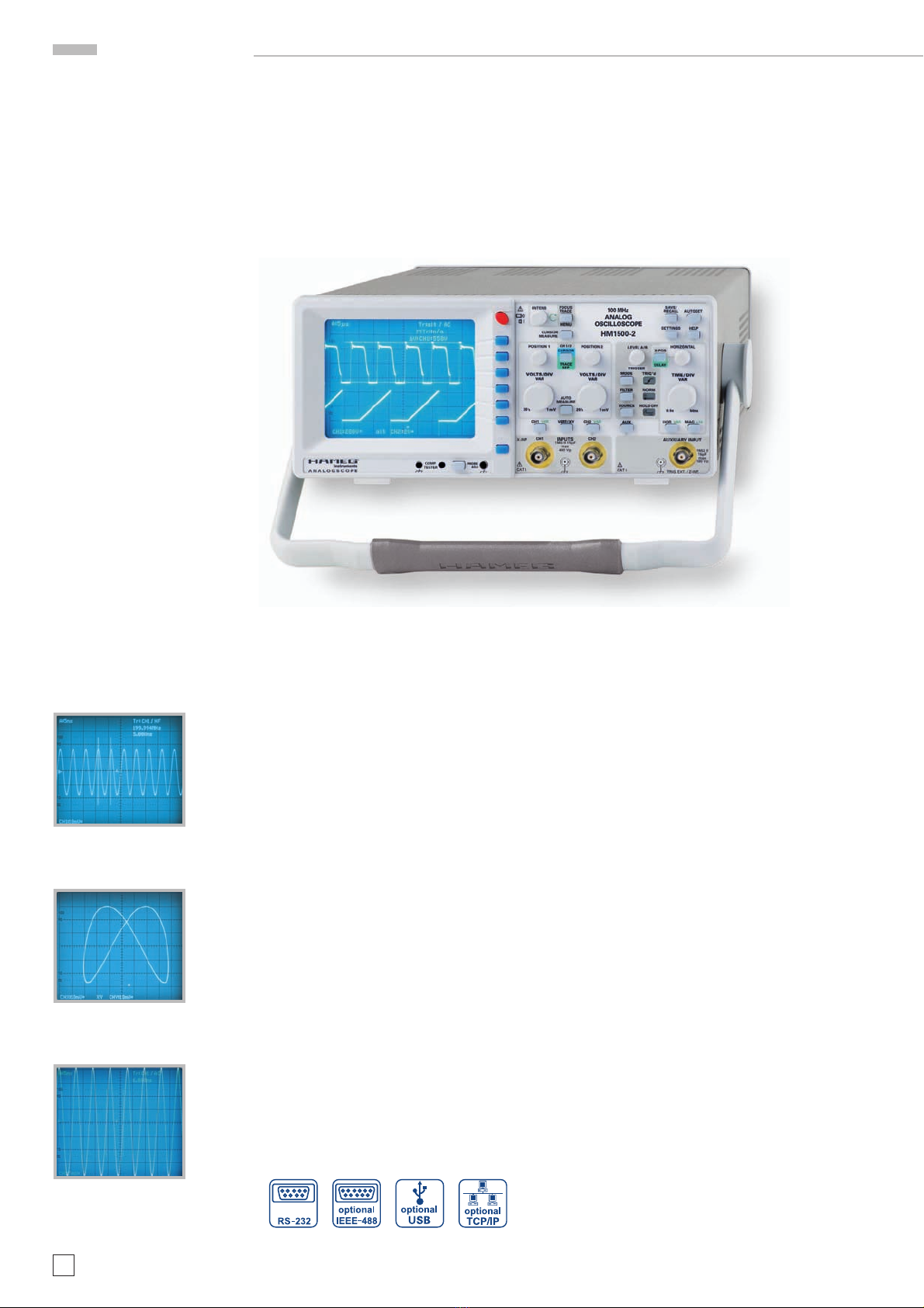
The oscilloscope HM1500-2 can display all repetitive signals
with a fundamental repetition frequency of at least 150MHz.
The frequency response is 0 to 150MHz (-3 dB). The vertical
amplifiers will not distort signals by overshoots, undershoots,
ringing etc.
Simple electrical signals like sine waves from line frequency
ripple to hf will be displayed without problems. However, when
measuring sine waves, the amplitudes will be displayed with
an error increasing with frequency. At 70MHz the amplitude
error will be around –10 %. As the bandwidths of individual
instruments will show a certain spread (the 150MHz are a
guaranteed minimum) the actual measurement error for sine
waves cannot be exactly determined.
Pulse signals contain harmonics of their fundamental frequency
which must be represented, so the maximum useful repetition
frequency of nonsinusoidal signals is much lower than 150MHz
(5 to 10 times). The criterion is the relationship between the rise
times of the signal and the scope; the scope’s rise time should
be <1/3 of the signal’s rise time if a faithful reproduction without
too much rounding of the signal shape is to be preserved.
The display of a mixture of signals is especially difficult if it
contains no single frequency with a higher amplitude than
those of the other ones as the scope’s trigger system normally
discriminates by amplitude. This is typical of burst signals for
example. Display of such signals may require using the HOLD-
OFF control.
Composite video signals may be displayed easily as the instru-
ment has a tv sync separator.
The maximum sweep speed of 5 ns/cm allows sufficient time
resolution, e.g. a 100MHz sine wave will be displayed one period
per 2 cm.
The vertical amplifier inputs may be DC or AC coupled. Use dc
coupling only if necessary and preferably with a probe.
Low frequency signals when AC coupled will show tilt (ac low
frequency – 3 dB point is 1.6 Hz), so if possible use DC coupling.
Using a probe with 10:1 or higher attenuation will lower the
–3 dB point by the probe factor. If a probe cannot be used due
to the loss of sensitivity, DC coupling the scope and an external
large capacitor may help which, of course, must have a sufficient
DC rating. Care must be taken, however, when charging and
discharging a large capacitor.
DC coupling is preferable with all signals of varying duty cycle,
otherwise the display will move up and down depending on the
duty cycle. Of course, pure DC can only be measured with DC
coupling. The readout will show which coupling was chosen:
= stands for DC, ~ stands for AC.
Amplitude of signals
In contrast to the general use of rms values in electrical en-
gineering oscilloscopes are calibrated in Vpp as that is what is
displayed. To derive rms from Vpp: divide by 2.84. To derive Vpp
from rms: multiply by 2.84.
Values of a sine wave signal
Vrms = rms value
Vpp = pp – value
Vmom = momentary value, depends on time vs period.
The minimum signal for a one cm display is 1 mVpp ±5 % provi-
ded 1 mV/cm was selected and the variable is in the calibrated
position.
The available sensitivities are given in mVpp or Vpp. The cursors
let you read the amplitudes of the signals immediately on the
readout as the attenuation of probes is automatically taken into
account. Even if the probe attenuation was selected manually
this will be overridden if the scope identifies a probe with an
identification contact as different. The readout will always give
the true amplitude.
It is important that the variable be in its calibrated position. The
sensitivity may be continuously decreased by using the variable
(see Controls and Readout). Each intermediate value between
the calibrated positions 1–2–5 may be selected. Without using
a probe thus a maximum of 400 VPP may be displayed (20 V/div
x 8 cm screen x 2.5 variable).
Amplitudes may be directly read off the screen by measuring
the height and multiplying by the V/div. setting.
STOP
Please note!
Without a probe the maximum permissible voltage
at the inputs must not exceed 400 Vp irrespective of
polarity.
In case of signals with a dc content the peak value DC + AC
peak must not exceed + or – 400 VP. Pure ac of up to 800 VPP
is permissible.
STOP
If probes are used their possibly higher ratings are
only usable if the scope is dc coupled.
In case of measuring DC with a probe while the scope input is
AC coupled the capacitor in the scope input will see the input
dc voltage as it is in series with the internal 1 MΩ resistor. This
means that the maximum dc voltage (or DC + peak AC) is that
of the scope input, i.e. 400 VP! With signals which contain DC
and AC the DC content will stress the input capacitor while
the AC content will be divided depending on the ac impedance
of the capacitor. It may be assumed that this is negligible for
frequencies >40 Hz.
Considering the foregoing you may measure DC signals of
up to 400 V or pure AC signals of up to 800 VPP with a HZ200
probe. Probes with higher attenuation like HZ53 100:1 allow
you to measure DC up to 1200 V and pure AC of up to 2400 VPP.
(Please note the derating for higher frequencies, consult the
HZ53 manual). Stressing a 10:1 probe beyond its ratings will
Basic signal measurement
VpVrms
Vmom
Vpp
Test Equipment Depot - 800.517.8431 - 99 Washington Street Melrose, MA 02176
FAX [phone] - TestEquipmentDepot.com

11
Subject to change without notice
risk destruction of the capacitor bridging the input resistor with
possible ensuing damage of the scope input!
If the residual ripple of a high voltage is to be measured, a high
voltage capacitor may be inserted in front of a 10:1 probe, it will
take most of the voltage as the value of the probe’s internal
capacitor is very low, 22 to 68 nF will be sufficient.
If the input selector is switched to Ground the reference trace
on the screen may be positioned at graticule center or else-
where.
DC and AC components of an input signal
The dashed curve shows an AC signal symmetrical to zero. If
there is a DC component the peak value will be DC + AC peak.
Timing relationships
The repetition frequency of a signal is equal to the number of
periods per second. Depending on the TIME/DIV setting one or
more periods or part of a period of the signal may be displayed.
The time base settings will be indicated on the readout in s/cm,
ms/cm, μs/cm und ns/cm (1 cm is equivalent to 1 div.). Also the
cursors may be used to measure the frequency or the period.
If portions of the signal are to be measured use delayed sweep
or the magnifier x 10. Use the HORIZONTAL positioning control
to shift the portion to be zoomed into the screen center.
Pulse signals are characterized by their rise and fall times
which are measured between the 10 % and 90 % portions. The
following example uses the internal graticule of the CRT, but
also the cursors may be used for measurement.
Measurement:
– Adjust the rising portion of the signal to 5 cm.
– Position the rising portion symmetrically to the graticule
centre line, using both Y and X positioning controls.
– Notice the intersections of the signal with the 10 and 90 %
lines and project these points to the centre line in order to
read the time difference.
In the example it was 1.6 cm at 5 ns/cm equals 8 ns rise time.
When measuring very short rise times times proceed mainly
as outlined above, however rise times may be measured any-
where on the screen. coming close to the scope rise time it is
necessary to subtract the scope’s (and if used the probe’s) rise
times geometrically from the rise time as seen on the screen.
The true signal rise time will become:
ttot is the rise time seen, tosc is the scope’s own rise time (2.3
ns with the HM1500-2), ttis the rise time of the probe, e.g. 2 ns.
If the signal’s rise time is >22 ns, the rise times of scope and
probe may be neglected.
For the measurement of rise times proceed mainly as outlined
above, however rise times may be measured anywhere on the
screen. It is mandatory that the rising portion of the signal be
measured in full and that the 10 to 90 % are observed. In case
of signals with over- or undershoot the 0 and 100 % levels are
those of the horizontal portions of the signal, i.e. the over- re-
spectively undershoots must be disregarded for rise and fall
time measurements. Also, glitches should be disregarded. If
signals are very distorted, however, rise and fall time measu-
rements may be of no value.
For most amplifiers, even if their pulse behaviour is far from
ideal, the following relationship holds:
350 350
ta=
—— B = ——
B ta
tr/ns = 350/Bandwidth/MHz
Connection of signals
In most cases pressing the AUTOSET button will yield a satis-
factory display (see AUTOSET). The following relates to special
cases where manual settings will be advisable. For a description
of controls refer to ”Controls and Readout“.
STOP
Take care when connecting unknown signals to the
inputs!
It is recommended to use probes whenever possible. Without
a probe start with the attenuator set to its 20 V/cm position. If
the trace disappears the signal amplitude may be too large,
overdriving the vertical amplifier or/and its dc content may
be too high. Reduce the sensitivity until the trace reappears
on screen. If calibrated measurements are desired it will be
necessary to use a probe if the signal becomes >160 Vp. Check
the probe specifications in order to avoid overstressing. If the
time base is set too fast the trace may become invisible, then
reduce the time base speed.
If no probe is used at least screened cable should be used,
such as HZ32 or HZ34. However, this is only advisable for low
impedance sources or low frequencies (<50 kHz). With high
frequencies impedance matching will be necessary.
Nonsinusoidal signals require impedance matching, at both
ends preferably. At the scope input a feed through – 50Ω-ter-
mination will be required. HAMEG offers a HZ22 termination. If
proper terminations are not used sizeable pulse aberrations will
Basic signal measurement
ta= 82- 2.32- 22= 7.4ns
ta= ttot2– tosc2– tt2
voltage
peak
AC
DC
DC
AC
DC + ACpeak = 400Vmax
5 cm
ttot
100%
90%
10%
0%

12 Subject to change without notice
result. Also sine wave signals of >100 kHz should be properly
terminated. Most generators control signal amplitudes only if
correctly terminated.
For loads (1 Watt; 7 Vrms or 20 Vpp) HAMEG offers the external
50Ω termination HZ22. For probes terminations are neither
required nor allowed, they would ruin the signal.
Probes feature very low loads at fairly low frequencies: 10 MΩ
in parallel to a few pF, valid up to several hundred kHz. How-
ever, the input impedance diminishes with rising frequency to
quite low values. This has to be borne in mind as probes are,
e.g., entirely unsuitable to measure signals across high impe-
dance high frequency circuits such as bandfilters etc.! Here
only FET probes can be used. Use of a probe as a rule will also
protect the scope input due to the high probe series resistance
(9MΩ). As probes cannot be calibrated precisely exactly enough
during manufacturing individual calibration with the scope input
used is mandatory! (See Probe Calibration).
Passive probes will, as a rule, decrease the scope bandwidth and
increase the rise time. We recommend to use HZ200 probes in
order to make maximum use of the combined bandwidth. HZ200
features 2 additional hf compensation adjustments.
Whenever the DC content is >400 VDC coupling must be used in
order to prevent overstressing the scope input capacitor. This is
especially important if a 100:1 probe is used as this is specified
for 1200 VDC + peak AC.
AC coupling of low frequency signals may produce tilt.
If the DC content of a signal must be blocked, it is possible to
insert a capacitor of proper size and voltage rating in front of the
probe, a typical application would be a ripple measurement.
When measuring small voltages the selection of the ground
connection is of vital importance. It should be as close to voltage
take off point as possible, otherwise ground currents may de-
teriorate the measurement. The ground connections of probes
are especially critical, they should be as short as possible and
of large surface area (litz wire; skin effect).
STOP
If a probe is to be connected to a BNC connector,
use a probe tip to BNC adapter.
If ripple or other interference is visible, especially at high sen-
sitivity, one possible reason may be multiple grounding. The
scope itself and most other equipment are connected to safety
ground, so ground loops may exist. Also, most instruments will
have capacitors between line and safety ground installed, which
conduct current from the live wire into the safety ground.
First time operation and initial adjustments
Prior to first time operation the connection between the instru-
ment and safety ground must be ensured, hence the plug must
be inserted first.
Use the red POWER pushbutton to turn the scope on. Several
displays will light up. The scope will then assume the set up,
which was selected before it was turned off. If no trace and
no readout are visible after approximately 20 sec, push the
AUTOSET button.
As soon as the trace becomes visible select an average inten-
sity with INTENS, then select FOCUS and adjust it, then select
TRACE ROTATION and adjust for a horizontal trace.
With respect to crt life, use only as much intensity as necessary
and convenient under given ambient light conditions. When not
in use, turn the intensity fully off rather than switching the scope
on and off too much as this is detrimental to the life of the crt
heater. Do not allow a stationary point on the screen, it might
burn the crt phosphor.
With unknown signals start with the lowest sensitivity 20 V/cm,
connect the input cables to the scope, and then to the measuring
object which should be de energized beforehand. Then turn the
measuring object on. If the trace disappears, push AUTOSET.
Trace rotation TR
The crt has an internal graticule. In order to adjust the deflected
beam with respect to this graticule the Trace Rotation control
is provided. Select the function Trace Rotation and adjust for a
trace which is exactly parallel to the graticule.
Probe adjustment and use
In order to ensure proper matching of the probe used to the
scope input impedance the oscilloscope contains a calibrator
with short rise time and an amplitude of 0.2 Vpp ±1 %, equivalent
to 4 cm at 5 mV/cm when using 10:1 probes.
The inner diameter of the calibrator connector is 4.9 mm and
standardized for series F probes. Using this special connec-
tor is the only way to connect a probe to a fast signal source
minimizing signal and ground lead lengths and to ensure true
displays of pulse signals.
1 kHz – adjustment
This basic adjustment will ensure that the capacitive attenuation
equals the resistive attenuation thus rendering the attenuation
of the probe independent of frequency. 1:1 probes can not be
adjusted and need no such adjustment anyway.
First time operation and initial adjustments
incorrect correct incorrect

13
Subject to change without notice
Operating modes of the vertical amplifier
The controls most important for the vertical amplifier are:
VERT/XY
28
, CH1 VAR
27
, CH2 VAR
29
. They give access to the
menus containing the operating modes and the parameters of
the individual channels.
Changing the operating mode is described in the chapter:
”Controls and Readout“.
Remark:
Any reference to ”both channels“ always refers to channels
1 and 2.
Usually oscilloscopes are used in the Yt mode.The amplitude
of the measuring signal will deflect the trace vertically while a
time base will deflect it from left to right.
The vertical amplifiers offer these modes:
– One signal only with CH1.
– One signal only with CH2.
− Two signals with channels 1 and 2 (DUAL trace mode)
− Two signals displayed as one in addition (ADD) mode
In DUAL mode both channels are operative. The method of
signal display is governed by the time base (see also ”Controls
and Readout“). Channel switching may either take place after
each sweep (alternate) or during sweeps at high frequency
(chopped).
The normal choice is alternate, however, at slow time base set-
tings the channel switching will become visible and disturbing,
when this occurs select the chopped mode in order to achieve
a stable quiet display.
In ADD mode the two channels 1 and 2 are algebraically ad-
ded (±CH1 ±CH2). With + polarity the channel is normal, with
– polarity inverted. If + Ch1 and – CH2 are selected the difference
will be displayed or vice versa.
Same polarity input signals:
Both channels not inverted: = sum
Both channels inverted: = sum
Only one channel inverted: = difference
Opposite polarity input signals:
Both channels not inverted: = difference
Both channels inverted: = difference
One channel inverted: = sum.
STOP
Please note that in ADD mode both position con-
trols will be operative. The INVERT function will not
affect positioning.
Often the difference of two signals is to be measured at signal
points which are both at a high common mode (CM) potential.
While this one typical application of the difference mode one
important precaution has to be borne in mind: The oscilloscope
vertical amplifiers are two separate amplifiers and do not con-
stitute a true difference amplifier with both a high CM rejection
and a high permissible CM range! Therefore please observe the
following rule: Always look at the two signals in the one channel
only or the dual modes (not in ADD mode) and make sure that
they are within the permissible input signal range; this is the
Prior to adjustment make sure that the trace rotation adjust-
ment has been performed.
Connect the 10:1 probe to the input. Use DC coupling. Set the
VOLTS/DIV knob for a signal height of 4 cm and TIME/DIV to 0.2
ms/cm, both calibrated. Insert the probe tip into the calibrator
connector PROBE ADJ.
You should see 2 signal periods. Adjust the compensation
capacitor (see the probe manual for the location) until the
square wave tops are exactly parallel to the graticule lines (see
picture 1 kHz). The signal height should be 4 cm ±1.6 mm (3%
oscilloscope and 1% probe tolerance). The rising and falling
portions of the square wave will be invisible.
1 MHz adjustment
The HAMEG probes feature additional adjustments in the
compensation box which allow to optimise their hf behaviour.
This adjustment is a precondition for achieving the maximum
bandwidth with probe and a minimum of pulse aberrations.
This adjustment requires a calibrator with a short rise time
(typ. 4 ns) and a 50Ω output, a frequency of 1 MHz, an amplitude
of 0.2 Vpp. The PROBE ADJ. output of the scope fulfils these
requirements.
Connect the probe to the scope input with which it is to be ad-
justed. Select the PROBE ADJ. signal 1MHz. Select dc coupling
and 5 mV/cm with VOLTS/DIV. and 0.1 us/cm with TIME/DIV.,
both calibrated. Insert the probe tip into the calibrator output
connector. The screen should show the signal, and the rise
and fall times will be visible. Watch the rising portion and the
top left pulse corner, consult the manual for the location of
the adjustments.
The criteria for a correct adjustment are:
– short rise time, steep slope.
– clean top left corner with minimum over- or undershoot,
flat top.
After adjustment check the amplitude which should be the
same as with 1 kHz.
It is important to first adjust 1 kHz, then 1 MHz. It may be ne-
cessary to check the 1 kHz adjustment again.
Please note that the calibrator signals are not calibrated with
respect to frequency and thus must not be used to check the
time base accuracy, also the duty cycle may differ from 1:1.The
probe adjustment is completed if the pulse tops are horizontal
and the amplitude calibration is correct.
Operating modes of the vertical amplifier
incorrect correct incorrect

14 Subject to change without notice
case if they can be displayed in these modes. Only then switch
to ADD. If this precaution is disregarded grossly false displays
may result as the input range of one or both amplifiers may
be exceeded.
Another precondition for obtaining true displays is the use of
two identical probes at both inputs. But note that normal probe
tolerances (percent) will cause the CM rejection to be expected
to be rather moderate. In order to obtain the best possible re-
sults proceed as follows: First adjust both probes as carefully
as possible, then select the same sensitivity at both inputs and
then connect both probes to the output of a pulse generator
with a sufficient amplitude to yield a good display. Readjust
one (!) of the probe adjustment capacitors for a minimum of
over- or undershoot. As there is no adjustment provided with
which the resistors can be matched a residual pulse signal will
be unavoidable.
When making difference measurements it is good practice
to first connect the ground cables of the probes to the object
prior to connecting the probe tips. There may be high potentials
between the object and the scope. If a probe tip is connected
first there is danger of overstressing the probe or/and the scope
inputs! Never perform difference measurements without both
probe ground cables connected.
XY operation
This mode is accessed by VERT/XY
28
>XY. In XY mode the
time base will be turned off. The channel 1 signal will deflect in
X direction (X-INP. = horizontal input) hence the input attenua-
tors, the variable and the POSITION 1 control will be operative.
The HORIZONTAL control will also remain functional.
Channel 2 will deflect in Y direction.
The x 10 magnifier will be inoperative in XY mode. Please note
the differences in the Y and X bandwidths, the X amplifier has
a lower –3dB frequency than the Y amplifier. Consequently
the phase difference between X and Y will increase with fre-
quency.
In XY mode the X signal (CH1 = X-INP) cannot be inverted.
The XY mode may generate Lissajous figures which simplify
some measuring tasks and make others possible:
– Comparison of two signals of different frequency or adjust-
ment of one frequency until it is equal to the other respec-
tively becomes synchronized.
– This is also possible for multiples or fractions of one of the
frequencies.
Phase measurements with Lissajous figures
The following pictures show two sine waves of equal amplitude
and frequency but differing phase.
Calculation of the phase angle between the X- and Y-signals (af-
ter reading a and b off the screen) is possible using the following
formulas and a pocket calculator with trigonometric functions.
This calculation is independent of the signal amplitudes:
Please note:
– As the trigonometric functions are periodic, limit the cal-
culation to angles <90 degrees. This is where this function
is most useful.
– Do not use too high frequencies, because, as explained
above, the two amplifiers are not identical, their phase
difference increases with frequency. The spec gives the
frequency at which the phase difference will stay <3 de-
grees.
– The display will not show which of the two frequencies does
lead or lag. Use a CR combination in front of the input of the
frequency tested. As the input has a 1 MΩ resistor it will be
sufficient to insert a suitable capacitor in series. If the ellipse
increases with the C compared to the C short circuited the
test signal will lead and vice versa. This is only valid <90
degrees. Hence C should be large and just create a barely
visible change.
If in XY mode, one or both signals may disappear, showing only
a line or a point, mostly very bright. In case of only a point there
is danger of phosphor burn, so turn the intensity down imme-
diately; if only a line is shown the danger of burn will increase
the shorter the line is. Phosphor burn is permanent.
Measurement of phase differences in dual channel
Yt mode
Please note: Do not use ”alternate trigger“ because the time
differences shown are arbitrary and depend only on the respec-
tive signal shapes! Make it a rule to use alternate trigger only
in rare special cases.
The best method of measuring time or phase differences is using
the dual channel Yt mode. Of course, only times may be read off
the screen, the phase must then be calculated as the frequency
is known. This is a much more accurate and convenient method
as the full bandwidth of the scope is used, and both amplifiers
are almost identical. Trigger the time base from the signal
which will be the reference. It is necessary to position both
traces without signal exactly on the graticule centre (POSITION
1 and 2). The variables and trigger level controls may be used,
this will not influence the time difference measurement. For
best accuracy display only one period at high amplitude and
observe the zero crossings. One period equals 360 degrees.
It may be advantageous to use ac coupling if there is an offset
in the signals.
Operating modes of the vertical amplifier
t = horizontal spacing of the
zero transitions in div
T= horizontal spacing for one
period in div
0° 35° 90° 180°
a b
a
sin ϕ=
—
b
a
cos ϕ= 1 –
(
—
)2
b
a
ϕ= arc sin
—
b

15
Subject to change without notice
In this example t = 3 cm and T = 10 cm, the phase difference in
degrees will result from:
5 3
ϕ° =
— ·360° = — ·360° = 108°
T 10
or in angular units:
t 3
arc ϕ° =
— · 2π= — · 2π= 1,885 rad
T 10
Very small phase differences with moderately high frequencies
may yield better results with Lissajous figures.
However, in order to get higher precision it is possible to switch
to higher sensitivities – after accurately positioning at graticule
centre , thus overdriving the inputs resulting in sharper zero
crossings. Also, it is possible to use half a period over the full
10 cm. As the time base is quite accurate, increasing the time
base speed after adjusting for e.g. one period = 10 cm and
positioning the first crossing on the first graticule line will also
give better resolution.
Measurement of amplitude modulation
The momentary amplitude at time t of an hf carrier frequency
modulated by a sinusoidal low frequency is given by:
u = UT·sinΩt + 0,5m ·UT·cos (Ω- ω) t - 0,5m ·UT·cos (Ω- ω) t
where: UT= amplitude of the unmodulated carrier
Ω= 2πF = angular carrier frequency
ω= 2πf = modulation angular frequency
m = modulation degree (≤1 v100%)
In addition to the carrier a lower side band F – f and an upper
side band F + f will be generated by the modulation.
Picture 1: Amplitudes and frequencies with AM (m = 50 %) of
the spectra
As long as the frequencies involved remain within the scope’s
bandwidth the amplitude-modulated hf can be displayed. Pre-
ferably the time base is adjusted so that several signal periods
will be displayed. Triggering is best done from the modulation
frequency. Sometimes a stable displayed can be achieved by
twiddling with the time base variable.
Picture 2: Amplitude modulated hf. F = 1 MHz, f = 1 kHz,
m = 50 %, UT= 28,3 mVrms
Set the scope controls as follows in order to display the picture
2 signal:
CH1 only, 20 mV/cm, AC
TIME/DIV: 0.2 ms/cm
Triggering: NORMAL, AC, internal.
Use the time base variable or external triggering.
Reading a and b off the screen the modulation degree will
result:
a – b a – b
m =
—— or m = —— ·100 [%]
a + b a + b
a = UT (1 + m) and b = UT(1 – m)
When measuring the modulation degree the amplitude and time
variables can be used without any influence on the result.
Operating modes of the vertical amplifier
F – f FF + f
0,5m · UT0,5m · UT
UT
ba
m · UT
UT
Test Equipment Depot - 800.517.8431 - 99 Washington Street Melrose, MA 02176
FAX [phone] - TestEquipmentDepot.com

16 Subject to change without notice
Triggering and time base
The most important controls and displays for these functions
are to be found in the shaded TRIGGER area, they are described
in „Controls and Readout“.-
In YT mode the signal will deflect the trace vertically while the
time will deflect it horizontally, the speed can be selected.
In general periodic voltage signals are displayed with a peri-
odically repeating time base. In order to have a stable display,
successive periods must trigger the time base at exactly the
same time position of the signal (amplitude and slope).
STOP
Pure DC can not trigger the time base, a voltage
change is necessary.
Triggering may be internal from any of the input signals or
externally from a time related signal.
For triggering a minimum signal amplitude is required which
can be determined with a sine wave signal. With internal trigge-
ring the trigger take off within the vertical amplifiers is directly
following the attenuators. The minimum amplitude is specified
in mm on the screen. Thus it is not necessary to give a minimum
voltage for each setting of the attenuator.
For external triggering the appropriate input connector is used,
thus the amplitude necessary there is given in Vpp. The voltage
for triggering may be much higher than the minimum, however,
it should be limited to 20 times the minimum. Please note that
for good triggering the external voltage should be a good deal
above the minimum. The scope features two trigger modes to
be described in the following:
Automatic peak triggering (MODE menu)
Consult the chapters MODE
16
>AUTO, LEVEL A/B
15
, FILTER
17
and SOURCE
18
in ”Controls and Readout“. Using AUTOSET
this trigger mode will be automatically selected. With DC coup-
ling and with alternate trigger this mode will be left while the
automatic triggering will remain.
Automatic triggering initiates a new time base start at the end
of each sweep, and after the hold off time has elapsed; even
without any input signal. Thus there is always a visible trace.
The position of the trace(s) without any signal is then given by
the settings of the POSITION controls.
As long as there is a signal, scope operation will not need more
than a correct amplitude and time base setting. With signals
<20 Hz their period is longer than the time the auto trigger
circuit will wait for a new trigger, consequently the auto trigger
circuit will start the time base irrespective of the signal. Hence
the display will not be triggered and free run, quite independent
of the signal’s amplitude which may be much larger than the
minimum.
Also in auto peak trigger mode, the trigger level control is active.
Its range will be automatically adjusted to coincide with the
signal’s peak to peak amplitude, hence the name. The trigger
point will thus become almost independent of signal amplitude.
This means that even if the signal is decreased the trigger will
follow, the display will not loose trigger. As an example: the
duty cycle of a square wave may change between 1:1 and 100:1
without loosing the trigger.
Depending on the signal the LEVEL A/B control may have to be
set to one of its extreme positions.
The simplicity of this mode recommends it for most uncompli-
cated signals. It is also preferable for unknown signals.
This trigger mode is independent of the trigger source and
usable as well for internal as external triggering. But the signal
must be >20 Hz.
Normal trigger mode (See menu MODE)
Consult the chapters: MODE
16
>AUTO, LEVEL A/B
15
, FILTER
17
and SOURCE
18
in ”Controls and Readout“. Tools for trigge-
ring very difficult signals can be found in the HOR VAR menu
26
where the functions time base fine adjustment VAR, HOLD OFF
time setting, and time base B operation are available.
With normal triggering and suitable trigger level setting, trigge-
ring may be chosen on any point of the signal slope. Here, the
range of the trigger level control depends on the trigger signal
amplitude. With signals <1 cm care is necessary.
In normal mode triggering there will be no trace visible in the
absence of a signal or when the signal is below the minimum
trigger amplitude requirement!
Normal triggering will function even with complicated signals. If
a mixture of signals is displayed triggering will require repetition
of amplitudes to which the level can be set. This may require
special care in adjustment.
Slope selection (Menu FILTER)
After entering FILTER
17
the trigger slope may be selected using
the function keys. See also ”Controls and Readout“. AUTOSET
will not change the slope.
Positive or negative slope may be selected in auto or normal
trigger modes. Also, a setting ”both“ may be selected which will
cause a trigger irrespective of the polarity of the next slope.
Rising slope means that a signal comes from a negative po-
tential and rises towards a positive one. This is independent
of the vertical position. A positive slope may exist also in the
negative portion of a signal. This is valid in automatic and
normal modes.
Trigger coupling (Menu: FILTER)
Consult chapters: MODE
16
>AUTO, LEVEL A/B
15
, FILTER
17
and SOURCE
18
in ”Controls and Readout“. In AUTOSET DC-
coupling will be used unless AC coupling was selected before.
The frequency responses in the diverse trigger modes may be
found in the specifications.
With internal DC coupling with or without LF filter use normal
triggering and the level control. The trigger coupling selected
will determine the frequency response of the trigger channel.
AC:
This is the standard mode. Below and above the fall off of the
frequency response more trigger signal will be necessary.
DC:
With direct coupling there is no lower frequency limit, so this
is used with very slowly varying signals. Use normal triggering
and the level control. This coupling is also indicated if the signal
varies in its duty cycle.
Triggering and time base

17
Subject to change without notice
HF:
A high pass is inserted in the trigger channel, thus blocking low
frequency interference like flicker, noise etc.
Noise Reject:
This trigger coupling mode or filter is a low pass suppressing
high frequencies. This is useful in order to eliminate hf inter-
ference of low frequency signals. This filter may be used in
combination with DC or AC coupling, in the latter case very low
frequencies will also be attenuated.
LF:
This is also a low pass filter with a still lower cut-off frequency
than above which also can be combined with dc or ac coupling.
Selecting this filter may be more advantageous than using DC-
coupling in order to suppress noise producing jitter or double
images. Above the pass band the necessary trigger signal will
rise. Together with ac coupling there will also result a low
frequency cut off.
Video (tv triggering)
Selecting MODE >Video will activate the built in TV sync se-
parator. It separates the sync pulses from the picture content
and enables thus stable triggering independent of the changing
video content.
Composite video signals may be positive or negative. The sync
pulses will only be properly extracted if the polarity is correct.
The definition of polarity is as follows: if the video is above the
sync it is positive, otherwise it is negative. The polarity can be
selected after selecting FILTER. If the polarity is wrong the
display will be unstable or not triggered at all as triggering will
then initiated by the video content. With internal triggering a
minimum signal height of 5 mm is necessary.
The PAL sync signal consists of line and frame signals which
differ in duration. Pulse duration is 5 μs in 64 μs intervals. Frame
sync pulses consist of several pulses each 28 μs repeating each
half frame in 20 ms intervals.
Both sync pulses differ in duration and in their repetition inter-
vals. Triggering is possible with both.
Frame sync pulse triggering
Remark:
Using frame sync triggering in dual trace chopped mode may
result in interference, then the dual trace alternate mode
should be chosen. It may also be necessary to turn the read-
out off.
In order to achieve frame sync pulse triggering call MODE,
select video signal triggering and then FILTER to select frame
triggering. It may be selected further whether ”all“, ”only even“
or ”only odd“ half frames shall trigger. Of course, the correct TV
standard must be selected first of all (625/50 or 525/60).
The time base setting should be selected to suit; with 2 ms/cm
a complete half frame will be displayed. Frame sync pulses
consist of several pulses with a half line rep rate.
Line sync pulse triggering
In order to choose line snyc triggering call MODE and select
VIDEO, enter FILTER, make sure that the correct video standard
is selected (625/50 or 525/60) and select Line.
If ”ALL“ was selected each line sync pulse will trigger. It is also
possible to select a line number ”LINE No.“.
In order to display single lines a time base setting of TIME/DIV.
= 10 μs/cm is recommended, this will show 1½ lines. In general
the composite video signal contains a high dc component which
can be removed by ac coupling, provided the picture is steady.
Use the POSITION control to keep the display within the screen.
If the video content changes such as with a regular tv program
only DC coupling is useful, otherwise the vertical position would
continuously move.
The sync separator is also operative with external triggering.
Consult the specifications for the permissible range of trigger
voltage. The correct slope must be chosen as the external
trigger may have a different polarity from the composite video.
In case of doubt display the external trigger signal.
LINE trigger
Consult SOURCE
18
in ”Controls and Readout“ for specific
information.
If the readout shows Tr:Line the trigger signal will be internally
taken from the line (50 or 60 Hz).
This trigger signal is independent of the scope input signals and
is recommended for all signals synchronous with the line. Within
limits this will also be true for multiples or fractions of the line
frequency. As the trigger signal is taken off internally there is
no minimum signal height on the screen for a stable display.
Hence even very small voltages like ripple or line frequency
interference can be measured.
Please note that with line triggering the polarity switching will
select either the positive or negative half period of the line, not
the slope. The trigger level control will move the trigger point
over most of a half wave.
Line frequency interference may be checked using a search
coil which preferably should have a high number of turns and
a shielded cable. Insert a 100Ω resistor between the center
conductor and the BNC connector. If possible the coil should
be shielded without creating a shorted winding.
Alternate trigger
This mode is selected with SOURCE
18
>Alt. 1/2. The readout
will display Tr:alt, but no trigger point symbol indicating level
and time position.
This trigger mode is to be used with greatest care and should be
an exception rather than the rule, because the time relationships
visible on the screen are completely meaningless, they depend
only on the shape of the signals and the trigger level!
In this mode the trigger source will be switched together with
the channel switching, so that when CH1 is displayed in the
dual channel alternate mode the trigger is taken from CH1
and when CH2 is displayed the trigger is taken from CH2. This
way two uncorrelated signals can be displayed together. If this
mode is inadvertently chosen the time relationships between
the signals will also be lost when both signals are correlated!
(Except for the special case that both happen to be square waves
with extremely fast rise times). Of course, this trigger mode is
only possible in the dual channel alternate mode and also not
with external or line trigger. AC coupling is recommended for
most cases.
Triggering and time base

18 Subject to change without notice
External triggering
This trigger mode may be selected with SOURCE
18
>Extern.
The readout will display Tr:ext. AUXILIARY INPUT
33
will be the
input for the external trigger signal, all internal trigger sources
will be disconnected. In this mode the trigger point symbol (level
and time position) will not be displayed, only the trigger time
position will be indicated. External triggering requires a signal
of 0.3 to 3 VPP, synchronous with the vertical input signal(s).
Triggering will also be possible within limits with multiples or
fractions of the vertical input signal frequency. As the trigger
signal may have any polarity, it may happen that the vertical
input signal will start with a negative slope in spite of having
selected positive slope; slope selection refers now to the ex-
ternal trigger.
Indication of triggered operation (TRIG’D LED)
Refer item
19
in ”Controls and Readout“. The LED labelled
TRIG’D indicates triggered operation provided:
– Sufficient amplitude of the internal or external trigger sig-
nal.
– The trigger point symbol is not above or below the signal.
If these conditions are met the trigger comparator will output
triggers to start the time base and to turn on the trigger indi-
cation. The trigger indicator is helpful for setting the trigger
up, especially with low frequency signals (use normal trigger)
and very short pulses.
The trigger indication will store and display triggers for 100 ms.
With signals of very low rep rate the indicator will flash accor-
dingly. If more than one signal period is shown on the screen
the indicator will flash each period.
Hold Off time adjustment
Consult ”Controls and Readout“ HOR VAR
26
>Hold off time
for specific information.
After the time base has deflected the trace from left to right,
the trace will be blanked so the retrace is invisible. The next
sweep will, however, not immediately start. Time is required
to perform internal switching, so the next start is delayed for
the so called hold off time, irrespective of the presence of
triggers. The hold off time can be extended from its minimum
by a factor of 10:1. Manipulation of the hold off time and thus
of the time for a complete sweep period from start to start can
be useful e.g. when data packets are to be displayed. It may
seem that such signals can not be triggered. The reason is
that the possible start of a new sweep does not coincide with
the start of a data packet, it may start anywhere, even before
a data packet. By varying the hold off time a stable display will
be achieved by setting it just so that the hold off ends before
the start of a data packet. This is also handy with burst signals
or non periodic pulse trains.
A signal may be corrupted by noise or hf interference so a double
display will appear. Sometimes varying the trigger level cannot
prevent the double display but will only affect the apparent time
relationship between two signals. Here the variable hold off time
will help to arrive at a single display.
Sometimes a double display will appear when a pulse signal
contains pulses of slightly differing height requiring delicate
trigger level adjustment. Also here increasing the hold off time
will help.
Whenever the hold off time was increased it should reset to its
minimum for other measurements, otherwise the brightness
will suffer as the sweep rep rate will not be maximum. The
following pictures demonstrate the function of the hold off:
period
heavy parts are displayed
signal
adjusting
HOLD OFF time
sweep
Fig. 1
Fig. 2
Picture 1: Display with minimum hold off time (basic setting).
Double image, no stable display.
Picture 2: By increasing the hold off a stable display is achie-
ved.
Time base B (2nd time base), Delaying, Delayed,
Sweep
Consult ”Controls and Readout“ HOR VAR
26
and TIME/DIV.
24
for specific information.
As was described in ”Triggering and time base“ a trigger will
start the time base. While waiting for a trigger, after runout of
the hold off time, the trace will remain blanked. A trigger will
cause trace unblanking and the sweep ramp which deflects
the trace from left to right with the speed set with TIME/DIV.
At the end of the sweep the trace will be blanked again and
reset to the start position. During a sweep the trace will also be
deflected vertically by the input signal. In fact the input signal
does continuously deflect the trace vertically, but this will be
only visible during the unblanking time.
Let us assume one period of a signal is displayed at a con-
venient time base setting. Increasing the sweep speed with
TIME/DIV. will expand the display from the start, so that parts
of the signal will disappear from the screen. It is thus possible
to expand the beginning of the signal period and show fine
detail, but it is impossible to show such fine detail for ”later“
parts of the signal.
The x10 Magnifier (MAG x10) may be used to expand the display
and the horizontal positioning control can shift any part of the
display into the centre, but the factor of 10 is fixed.
The solution requires a second time base, called time base B.
In this mode time base A is called the delaying sweep and
time base B the delayed sweep. The signal is first displayed
by TB A alone. Then TB B is also turned on which is the mode
”A intensified by B“. TB B should always be set to a higher sweep
rate than A, thus its sweep duration will be also shorter than
that of A. The TB A sweep sawtooth is compared to a voltage
Triggering and time base

19
Subject to change without notice
AUTOSET
For specific information consult ”Controls and Readout“
AUTOSET
7
.
AUTOSET enables a standard automatic instrument setting, if
the applied signal meets the amplitude and frequency require-
ments of automatic triggering.
All controls except for the POWER switch are electronically
scanned and therefore can also be controlled by the micro-
computer.
This is a precondition for AUTOSET as this function must be able
to control all functions independent of control settings. AUTO-
SET will always switch to YT mode, but preserve the previous
selection of CH1, CH2 or dual trace; ADD or XY modes will be
switched to dual trace Yt.
Automatic setting of the vertical sensitivities and the time base
will present a display within 6 cm height (4 cm per signal in dual
trace) and about 2 signal periods. This is true for signals not
differing too much from a 1:1 duty cycle. For signals containing
several frequencies like video signals the display may be any.
Initiating the AUTOSET function will set the following operating
conditions:
– last selection of AC or DC coupling
– internal triggering
– automatic triggering
– trigger level set to the center of its range
– calibrated Y sensitivities
– calibrated time base
– AC or DC trigger coupling unmodified
– HF trigger coupling switched to DC
– LF or Noise Reject filters left
– X magnifier switched off
– Y and X positioning automatic
Please note:
For pulse signals with duty cycles approaching 400:1 no au-
tomatic signal display will be possible.
In such cases switch to normal trigger mode and set the trigger
position about 5 mm above the centre. If the trigger LED will then
light up a trigger is generated and the time base is operating. In
order to obtain a visible display it may be necessary to change
the time base and V/DIV settings. Depending on the duty cycle
and the frequency the signal may still remain invisible.
which can be varied such that TB A functions as a precision
time delay generator. Depending on the amplitude of the com-
parison voltage a signal is generated anywhere between sweep
start and end.
In one of two operating modes this signal will start TB B imme-
diately. The TB A display will be intensified for the duration of
TB B, so that one sees which portion of the signal is covered by
TB B. By varying the comparison voltage the start of TB B can
be moved over the whole signal as it is displayed by TB A. Then
the mode is switched to TB B. The signal portion thus selected is
now displayed by TB B. This is called „B delayed by A“. Portions
of the signal can thus be expanded enormously, however, the
higher the speed of TB B, the darker the display will become,
the rep rate will remain that of the input trigger signal triggers
while the duration of TB B is reduced with increasing speed.
The readout display is not affected.
In cases where there is jitter the TB B can be switched to wait
for a trigger rather than starting immediately. When a trigger
arrives TB B will be started on it. The jitter is removed, however,
the effect is also, that the TB B start now can be only from signal
period to signal period, no continuous adjustment is possible
in this mode.
Alternate sweep
In this mode the signal is displayed twice, with both time bases.
An artificial Y offset can be added in order to separate the two
displays on the screen. The operation is analogous to Y dual
trace alternate mode, i.e., the signal is alternately displayed by
both time bases, not simultaneously which is not possible with
a single gun crt. TB B operation is the same here.
Triggering and time base

20 Subject to change without notice
Component tester
Specific information can be found in ”Controls and Readout“ un-
der COMPONENT/PROBE
35
and COMPONENT TESTER
36
.
The scope has a built-in component tester. The test object is
connected with 4 mm banana plugs. In this mode the Y amplifiers
and the time base are turned off. Only individual components
may be tested, i.e. they must not be part of a circuit, if voltages
are to be applied to the BNC connectors. If the components are
part of a circuit this must be de-energized and disconnected
from safety ground. Except for the two test leads there may
be no further connection between scope and component. (See
”Tests within a circuit“). As described in section ”Safety“ all
ground connections of the scope are connected to safety ground
including those of the component tester. As long as individual
components are tested this is of no consequence.
The display can only be affected by the controls contained in
the FOCUS/TRACE menu: A-Int., Focus, Trace rotation, HORI-
ZONTAL position.
If components are to be tested which are parts of a circuit or
an instrument those circuits respectively instruments must
first be de-energized. If they are connected to the mains they
must be unplugged. This will prevent a connection between
scope and circuit via the safety ground which may affect the
measurement.
STOP
Do not test charged capacitors.
The principle of the test is very simple: a sine wave generator
within the scope generates a 50 Hz ±10 % voltage which is
applied to a series connection of the test object and a resistor
within the scope. The sine wave proper deflects in X direction,
the voltage across the resistor which is proportional to the test
current deflects in Y direction.
If the object contains neither capacitors nor inductors, there will
be no phase shift between voltage and current, so a straight
line will show up which will be more or less slanted, depending
on the value of the object’s resistance, covering appr. 20Ω to
4.7 kΩ. If there is a short the trace will be vertical, i.e. (almost)
no voltage produces already high current. A horizontal line will
thus indicate an open, there is only voltage but no current.
Capacitors or inductors will create ellipses. The impedance
may be calculated from the ellipse’s geometric dimensions.
Capacitors of approx. 0.1μ to 1000 μF will be indicated.
– An ellipse with its longer axis horizontal indicates a high
impedance (low capacitance or high inductance)
– An ellipse with its longer axis vertical will indicate a low
impedance (high capacitance or low inductance)
– A slanted ellipse will indicate a lossy capacitor or induc-
tor.
Semiconductors will show their diode characteristics, however,
only 20 Vpp are available, so the forward and reverse characte-
ristics can only be displayed up to 10 Vpin each direction. The
test is a two-terminal test ,hence it is not possible to measure
e.g. the current gain of a transistor. One can only test B-C, B-E,
and C-E. The test current is only a few mA, so the test will not
harm ordinary semiconductors. (Sensitive devices like delicate
hf transistors etc. should not be tested). The limitation to 10
Component tester
Vp with bipolar transistors will suffice mostly as usual defects
will show up.
STOP
Attention: Before testing a component, please
check its data to ensure that it would not be over-
loaded by the test voltage of ± 10 V.
The best method to verify whether a component is defective is
the comparison to a good one. If the lettering of a component
is not legible at least it is possible to see whether it is a npn or
pnp transistor or which end of a diode is the cathode.
Please note that reversing the test leads will also invert the
picture, i.e. turn it 180 degrees.
In most cases, e.g. with service and repair, it will be sufficient
to receive a good/bad result (open, short). With MOS compo-
nents the usual precautions are to be observed, but note, that
except for a possible short MOSFETs and JFETs can not be
sufficiently tested. Indications to be expected depend strongly
on the kind of FET:
– With depletion type MOSFETs and all JFETs the channel
will conduct if prior to testing the gate was connected to the
source. The Rdson will be shown. As this can be very low it
may look like a plain short although the part is good!
– With enhancement type MOSFETs an open will be seen in
all directions, as the threshold voltage G – S is not available.
With power MOSFETs the anti parallel diode S – D can be
seen.
Tests of components within circuits are possible in many cases
but less indicative because other components may be in parallel.
But also here the comparison with a good circuit might help. As
both circuits must be deenergized it is only necessary to switch
the test leads back and forth between both in order to localize
a defective spot. Sometimes like with stereo amplifiers, push-
pull circuits, bridge circuits there is a comparison circuit right
on the same board. In cases of doubt one component lead can
be unsoldered, the other one should then be connected to the
ground lead. This is labelled with a ground symbol. The pictures
show some practical examples.
Test Equipment Depot - 800.517.8431 - 99 Washington Street Melrose, MA 02176
FAX [phone] - TestEquipmentDepot.com